Ocean framework
The ocean core contains a small amount of shared framework code that we
expect to expand in the future as new test cases are added.
Namelist replacements and streams files
The modules compass.ocean.namelists and compass.ocean.streams contain
namelist replacements and streams files that are similar to core-level
templates in Legacy COMPASS. Current templates are for adjusting sea
surface height in ice-shelf cavities, and outputting variables related to
frazil ice and land-ice fluxes.
Vertical coordinate
The compass.ocean.vertical module provides support for computing general
vertical coordinates for MPAS-Ocean test cases.
The compass.ocean.vertical.grid_1d module provides 1D vertical
coordinates. To create 1D vertical grids, test cases should call
compass.ocean.vertical.grid_1d.generate_1d_grid() with the desired
config options set in the vertical_grid section (as described in
Vertical coordinate).
The z-level and z-star coordinates are also controlled by config options from
this section of the config file. The function
compass.ocean.vertical.init_vertical_coord() can be used to compute
minLevelCell, maxLevelCell, cellMask, layerThickness, zMid,
and restingThickness variables for z-level and
z-star coordinates using the ssh and bottomDepth as well
as config options from vertical_grid.
Haney number
The module compass.ocean.haney defines a function
compass.ocean.haney.compute_haney_number() for computing the Haney
number (Haney 1991).
The Haney number is a measure of how large pressure-gradient errors are likely
to be based on how thin and tilted the model layers have become.
where the computation is centered at edge \(e\) and at the interface between layers \(k\) and \(k+1\), adjacent to cells \(c_1\) and \(c_2\). The elevation of the middle of layer \(k\) at the center of cell \(c\) is \(z_\textrm{mid}(c, k)\).
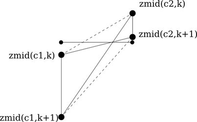
The locations of four adjacent cell centers used in the computation of the Haney number (and the horizontal pressure-gradient force).
Ice-shelf cavities
The module compass.ocean.iceshelf defines two functions that are used to
set up domains with ice-shelf cavities.
compass.ocean.iceshelf.compute_land_ice_pressure_and_draft()
computes the landIcePressure and landIceDraft fields based on the
sea-surface height (SSH) and a reference density (typically the the Boussinesq
reference density).
compass.ocean.iceshelf.adjust_ssh() performs a series of forward
runs with MPAS-Ocean to detect and correct imbalances between the SSH and the
land-ice pressure. In each forward run, the SSH is allowed to evolve forward
in time for a short period (typically 1 hour), then the resulting change in
SSH is translated into a compensating change in land-ice pressure that is
expected to reduce the change in SSH. The initial land-ice pressure is updated
accordingly and the process is repeated for a fixed number of iterations,
typically leading to smaller and smaller changes in the land-ice pressure.
This process does not completely eliminate the dynamical adjustment of the
ocean to the overlying weight of the ice shelf but it tends to reduce it
substantially and to prevent it from causing numerical instabilities. This
procedure is also largely agnostic to the equation of state being used or the
method for implementing the horizontal pressure-gradient force.
Particles
The compass.ocean.particles module contains functionality for initializing
particles for the LIGHT framework.
compass.ocean.particles.write() creates an initial condition for
particles partitioned across cores. There are 3 possible particle types (or
all to indicate that all 3 types will be generated):
buoyancyParticles are constrained to buoyancy (isopycnal) surfaces
passiveParticles move both horizontally and vertically as passive tracers
surfaceParticles are constrained to the top ocean level
compass.ocean.particles.remap_particles() is used to remap particles
onto a new grid decomposition. This might be useful, for example, if you wish
to change the number of cores that a particle initial condition should run on.
Plotting
The compass.ocean.plot contains functionality for plotting the initial
state and 1D vertical grid.
compass.ocean.plot.plot_initial_state() creates histogram plots of
salinity, temperature, bottom depth, maxLevelCell, layer thickness and the
Haney number from global initial condition. This is useful for providing a
quick sanity check that these values have the expected range and distribution,
based on previous meshes.
compass.ocean.plot.plot_vertical_grid() plot the vertical grid in
3 ways: layer mid-depth vs. vertical index; layer mid-depth vs. layer thickness;
and layer thickness vs. vertical index. Again, this provides a quick sanity
check that the grid has the expected bounds (both in thickness and in depth)
and number of layers.