Visualization
Plotting Landice Transects
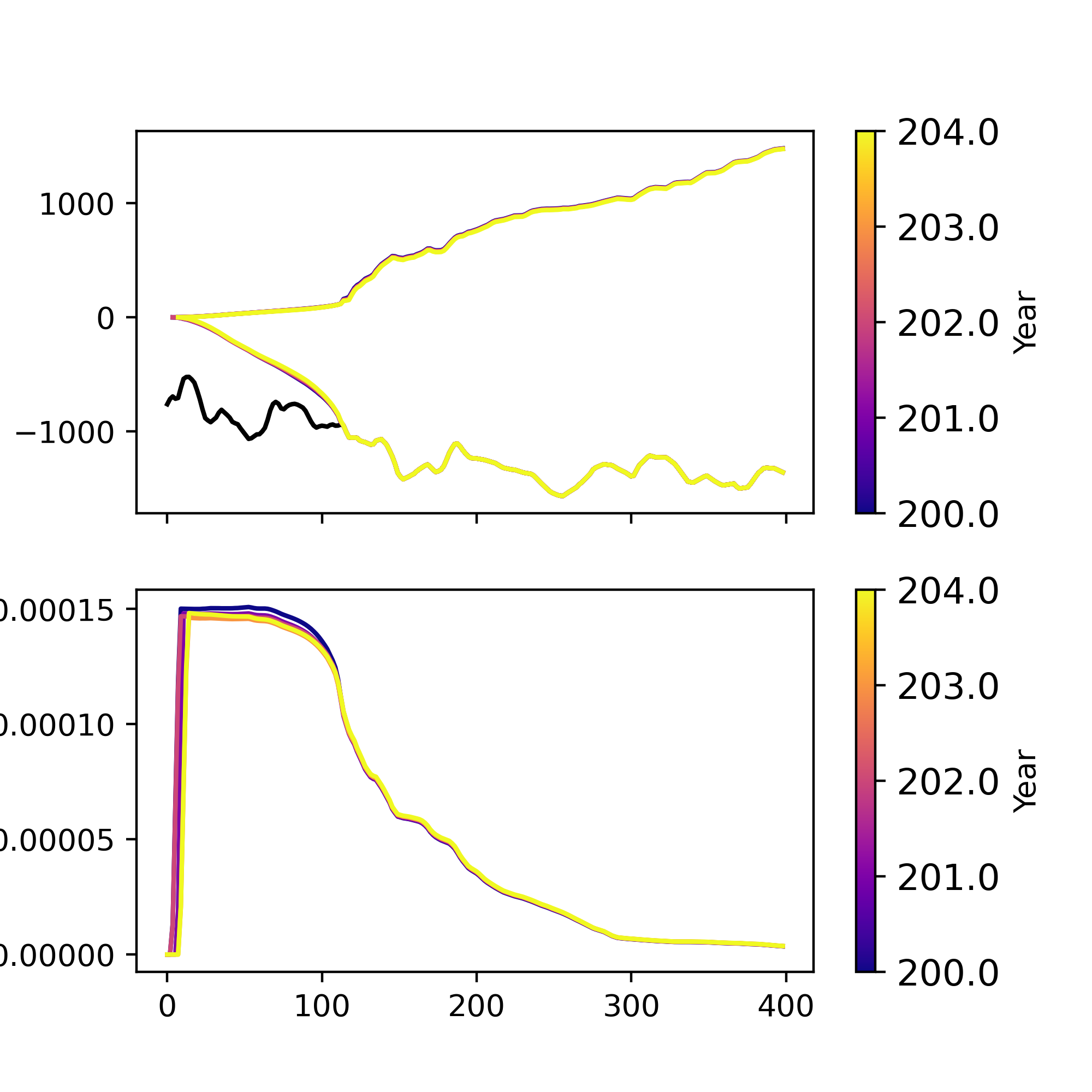
The function mpas_tools.landice.visualization.plot_transect() can be
used to plot transects of various cell-centered MALI variables. The above figure
was plotted with the code:
import matplotlib.pyplot as plt
from netCDF4 import Dataset
from mpas_tools.landice.visualization import plot_transect


fig, ax = plt.subplots(2,1, figsize=(5,5), sharex=True)
data_path = "ISMIP6/archive/expAE02/"
file = "2200.nc"
x = [-1589311.171,-1208886.353]
y = [-473916.7182,-357411.6176]
times = [0, 1, 2, 3, 4]
plot_transect(data_path + file, "geometry", ax=ax[0], times=times,  x=x, y=y)
plot_transect(data_path + file, "surfaceSpeed", ax=ax[1], times=times,  x=x, y=y)
fig.savefig("thwaites_transect.png", dpi=400)
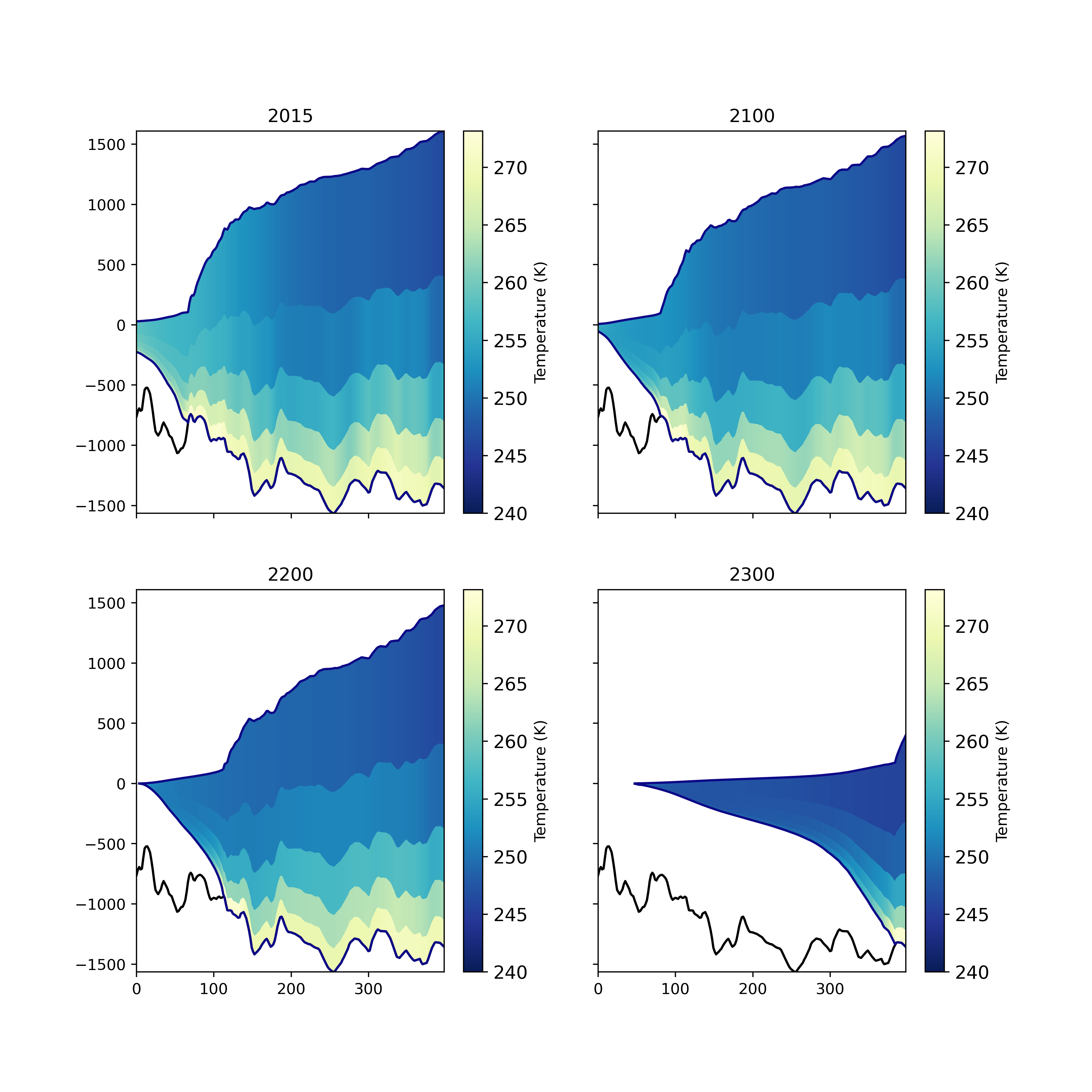
This can also be used to produce transects of ice temperature, with one time level should be plotted per subplot:
fig, axs = plt.subplots(2,2, figsize=(10,10), sharex=True, sharey=True)
files = ["rst.2015-01-01.nc", "rst.2100-01-01.nc", "rst.2200-01-01.nc", "rst.2300-01-01.nc"]
x = [-1589311.171,-1208886.353]
y = [-473916.7182,-357411.6176]

for ax, file in zip(axs.ravel(), files):
    plot_transect(data_path + file, "temperature", ax=ax,
                  times=[0], x=x, y=y)
    ax.set_title(file[4:8])
fig.savefig("thwaites_temperature_transects.png", dpi=400)
Plotting Landice Maps
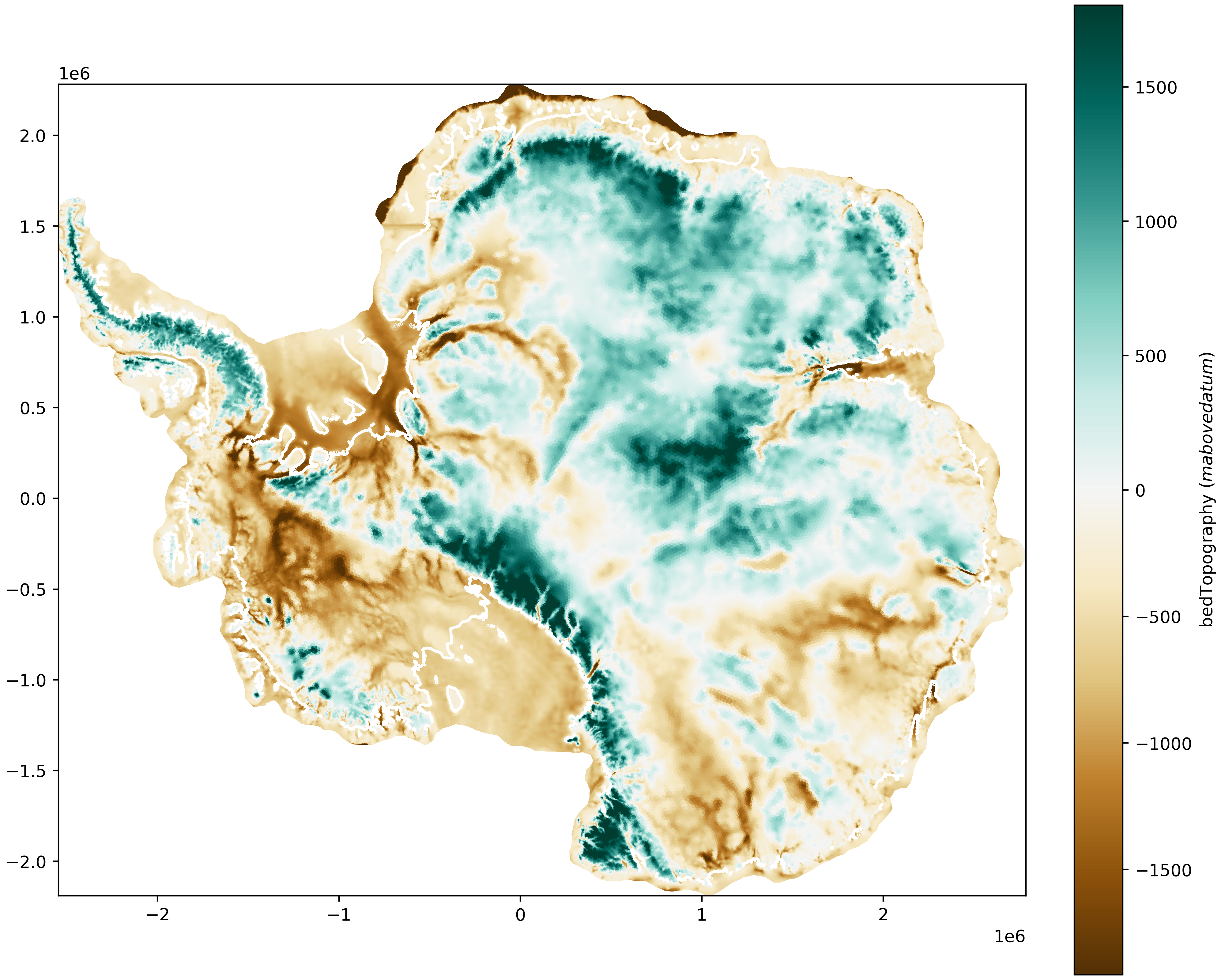
The function mpas_tools.landice.visualization.plot_map() can be
used to plot maps of cell-centered MALI variables. The above
figure was plotted using:
from mpas_tools.landice.visualization import plot_map


fig, ax = plt.subplots(1, 1, figsize=(10,8), layout='constrained')
var_plot, cbar, gl_plot = plot_map(data_path + files[0], "bedTopography",
                                   ax=ax, time=0, plot_grounding_line=True)
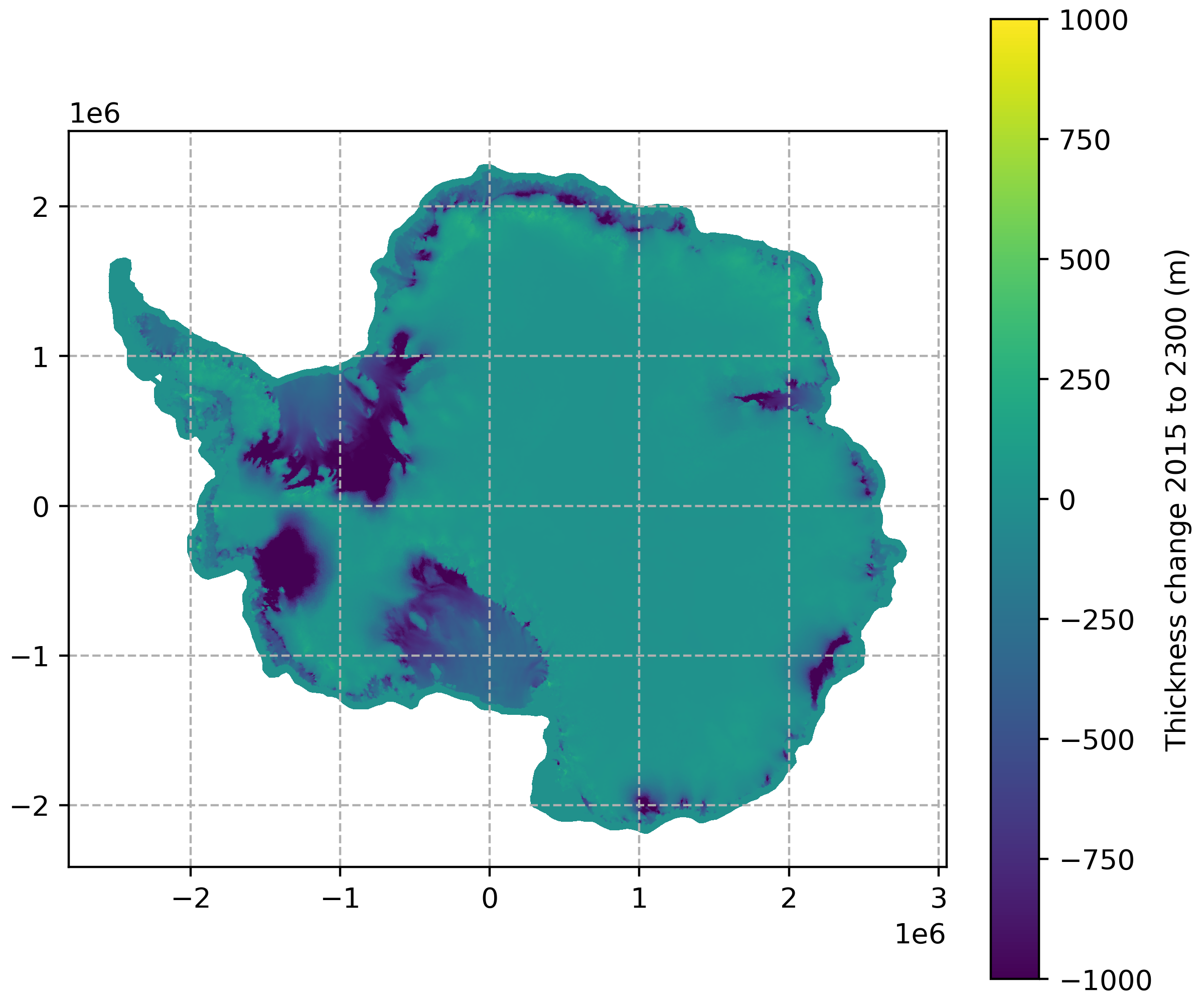
This can also be used to plot derived fields, such as thickness change from 2015 to 2300:
data_2300 = Dataset(data_path + "output_state_2300.nc")
data_2300.set_auto_mask(False)
data_2015 = Dataset(data_path + "output_state_2015.nc")
data_2015.set_auto_mask(False)
thk_2300 = data_2300.variables["thickness"][:]
thk_2015 = data_2015.variables["thickness"][:]

fig, ax = plt.subplots(1, 1, figsize=(6,5), layout='constrained')
thk_diff_plot, thk_diff_cbar, _ = plot_map(
    data_path + "output_state_2015.nc", variable=thk_2300-thk_2015,
    ax=ax, time=0, vmin=-1000, vmax=1000, plot_grounding_line=False,
    variable_name="Thickness change 2015 to 2300 (m)")
ax.grid(linestyle='dashed')
Plotting Landice Grounding Lines
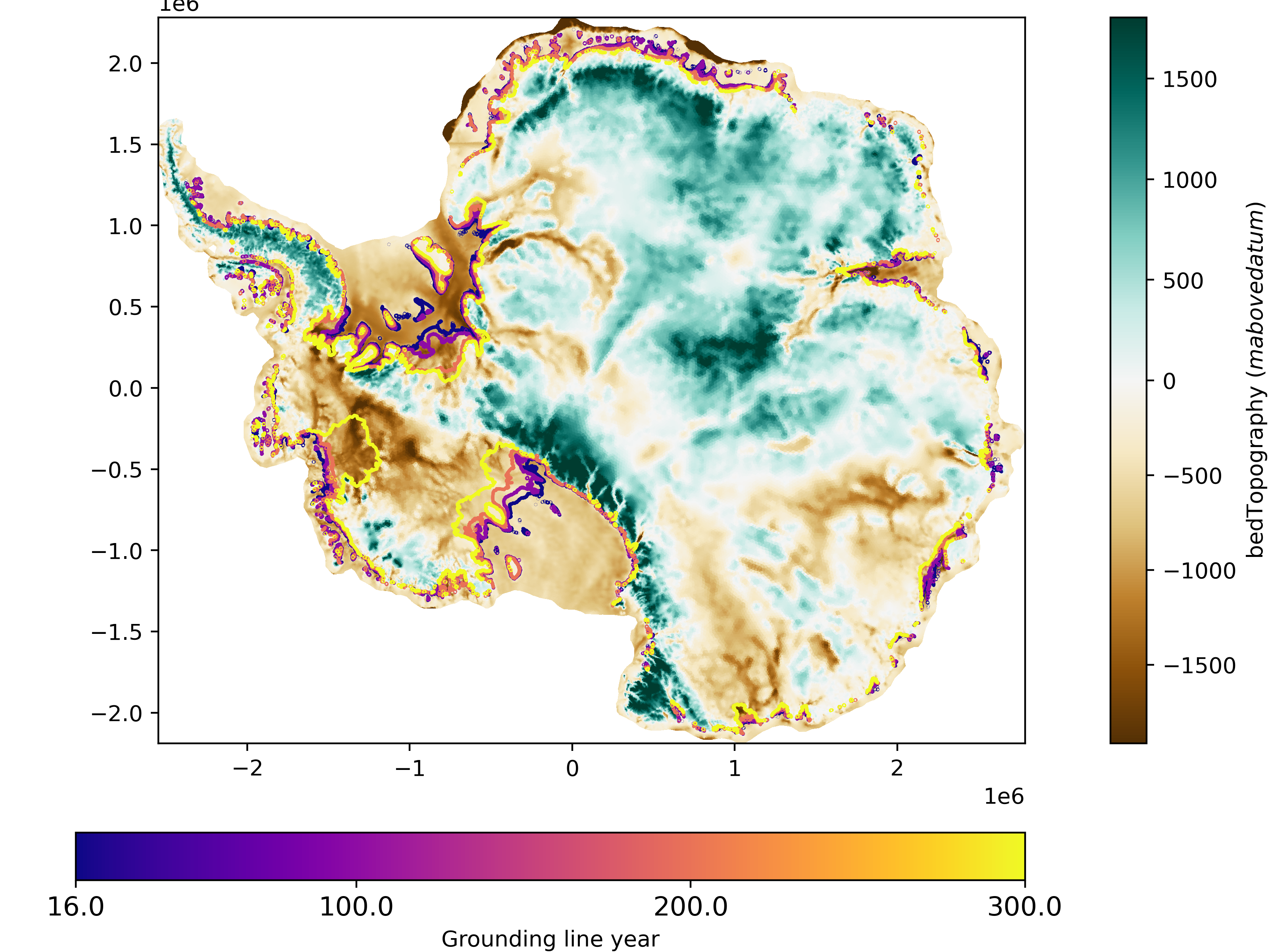
The function mpas_tools.landice.visualization.plot_grounding_lines() can be
used to add grounding lines to maps as countours.
from mpas_tools.landice.visualization import plot_grounding_lines


fig, ax = plt.subplots(1, 1, figsize=(8,6), layout='constrained')
plot_grounding_lines([data_path + "output_state_2015.nc",
                      data_path + "output_state_2100.nc",
                      data_path + "output_state_2200.nc",
                      data_path + "output_state_2300.nc"],
                     ax=ax,
                     cmap="plasma", times=[0])
plot_map(data_path + files[0], "bedTopography", ax=ax, time=0)