oceanRegionalProfiles

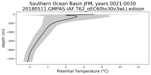
An analysis task for plotting depth profiles of temperature, salinity, potential density, etc. averaged over regions and in time. The plots also include a measure of variability (the standard deviation in space and time).

Component and Tags:

component: ocean
tags: profiles, climatology

Configuration Options

The following configuration options are available for this task:

[oceanRegionalProfiles]
## options related to plotting vertical profiles of regional means (and
## variability) of 3D MPAS fields

# a list of dictionaries for each field to plot.  The dictionary includes
# prefix (used for file names, task names and sections) as well as the mpas
# name of the field, units for colorbars and a the name as it should appear
# in figure titles and captions.
fields =
    [{'prefix': 'temperature',
      'mpas': 'timeMonthly_avg_activeTracers_temperature',
      'units': r'$\degree$C',
      'titleName': 'Potential Temperature'},
     {'prefix': 'salinity',
      'mpas': 'timeMonthly_avg_activeTracers_salinity',
      'units': r'PSU',
      'titleName': 'Salinity'},
     {'prefix': 'potentialDensity',
      'mpas': 'timeMonthly_avg_potentialDensity',
      'units': r'kg m$^{-3}$',
      'titleName': 'Potential Density'}]

# Times for comparison times (Jan, Feb, Mar, Apr, May, Jun, Jul, Aug, Sep, Oct,
# Nov, Dec, JFM, AMJ, JAS, OND, ANN)
seasons =  ['JFM', 'JAS', 'ANN']

# minimum and maximum depth of profile plots, or empty for the full depth range
depthRange = []

# The suffix on the regional mask file to be used to determine the regions to
# plot.  A region mask file should be in the regionMaskDirectory and should
# be named <mpasMeshName>_<regionMaskSuffix>.nc
regionMaskSuffix = oceanBasins

# a list of region names from the region masks file to plot
regionNames = ["Atlantic_Basin", "Pacific_Basin", "Indian_Basin",
               "Arctic_Basin", "Southern_Ocean_Basin", "Mediterranean_Basin",
               "Global Ocean", "Global Ocean 65N to 65S",
               "Global Ocean 15S to 15N"]

# Make Hovmoller plots of fields vs time and depth?
plotHovmoller = False

# web gallery options
hovmollerGalleryGroup = Ocean Basin Time Series vs Depths

# web gallery options
profileGalleryGroup = Ocean Basin Profiles


[temperatureOceanRegionalHovmoller]
## options related to plotting time series of temperature vs. depth in ocean
## regions

# Number of points over which to compute moving average(e.g., for monthly
# output, movingAveragePoints=12 corresponds to a 12-month moving average
# window)
movingAveragePoints = 1

# colormap
colormapName = RdYlBu_r
# whether the colormap is indexed or continuous
colormapType = continuous
# the type of norm used in the colormap
normType = linear
# A dictionary with keywords for the norm
normArgs = {'vmin': -2., 'vmax': 30.}

# contour line levels (use [] for automatic contour selection, 'none' for no
# contour lines)
contourLevels = 'none'

# An optional first year for the tick marks on the x axis. Leave commented out
# to start at the beginning of the time series.

# firstYearXTicks = 1

# An optional number of years between tick marks on the x axis.  Leave
# commented out to determine the distance between ticks automatically.

# yearStrideXTicks = 1

# limits on depth, the full range by default
# yLim = [-6000., 0.]


[salinityOceanRegionalHovmoller]
## options related to plotting time series of salinity vs. depth in ocean
## regions

# Number of points over which to compute moving average(e.g., for monthly
# output, movingAveragePoints=12 corresponds to a 12-month moving average
# window)
movingAveragePoints = 1

# colormap
colormapName = haline
# whether the colormap is indexed or continuous
colormapType = continuous
# the type of norm used in the colormap
normType = linear
# A dictionary with keywords for the norm
normArgs = {'vmin': 30, 'vmax': 39.0}

# contour line levels (use [] for automatic contour selection, 'none' for no
# contour lines)
contourLevels = 'none'

# An optional first year for the tick marks on the x axis. Leave commented out
# to start at the beginning of the time series.

# firstYearXTicks = 1

# An optional number of years between tick marks on the x axis.  Leave
# commented out to determine the distance between ticks automatically.

# yearStrideXTicks = 1

# limits on depth, the full range by default
# yLim = [-6000., 0.]


[potentialDensityOceanRegionalHovmoller]
## options related to plotting time series of potential density vs. depth in
## ocean regions

# Number of points over which to compute moving average(e.g., for monthly
# output, movingAveragePoints=12 corresponds to a 12-month moving average
# window)
movingAveragePoints = 1

# colormap
colormapName = Spectral_r
# whether the colormap is indexed or continuous
colormapType = continuous
# the type of norm used in the colormap
normType = linear
# A dictionary with keywords for the norm
normArgs = {'vmin': 1026.5, 'vmax': 1028.}

# contour line levels (use [] for automatic contour selection, 'none' for no
# contour lines)
contourLevels = 'none'

# An optional first year for the tick marks on the x axis. Leave commented out
# to start at the beginning of the time series.

# firstYearXTicks = 1

# An optional number of years between tick marks on the x axis.  Leave
# commented out to determine the distance between ticks automatically.

# yearStrideXTicks = 1

# limits on depth, the full range by default
# yLim = [-6000., 0.]

The fields dictionary is used to specify a list of 3D MPAS fields to average and plot. The key prefix is a convenient name appended to tasks and file names to describe the field. mpas is the name of the field in MPAS timeSeriesStatsMonthly output files. The units are the SI units of the field to include on the plot’s x axis and titleName is the name of the field to use in its gallery name and on the x axis of the profile.

The option regionMaskSuffix is a suffix for files and tasks describing the set of regions being plotted. The file <regionMaskSuffix>.geojson should exist in regionMasksSubdirectory.

regionNames is a list of regions from the full list of regions in <regionMaskSuffix>.geojson or regionNames = ['all'] to indicate that all regions should be used.

The task can be used to produce Hovmoller plots of each field averaged over each region. By default, these plots are disabled by can be enabled by setting plotHovmoller = True. The sections [<prefix>OceanRegionalHovmoller] give options for these Hovmoller plots.

Config options are availabe to specify the names of the gallery group for the profiles (profileGalleryGroup) and Hovmoller plots (hovmollerGalleryGroup) if the latter are plotted.

A minimum and maximum depth for profiles can be specified with depthRange. Similarly, each section for displaying Hovmoller plots of each field has a yLim option that can specify the desired depth range. In all cases, the default is the full range.

For more details on the remaining config options, see

• Regions

• Seasons

• Colormaps

• Moving Average

• Time-Axis Tick Marks

Example Result