baroclinic_gyre

The baroclinic_gyre test group implements variants of the baroclinic ocean gyre set-up from the MITgcm test case.

This test simulates a baroclinic, wind and buoyancy-forced, double-gyre ocean circulation. The grid employs spherical polar coordinates with 15 vertical layers. The configuration is similar to the double-gyre setup first solved numerically in Cox and Bryan (1984): the model is configured to represent an enclosed sector of fluid on a sphere, spanning the tropics to mid-latitudes, ${60}^{\circ }\times {60}^{\circ }$ in lateral extent. The fluid is $1.8$km deep and is forced by a zonal wind stress which is constant in time, ${\tau }_{\lambda }$, varying sinusoidally in the north-south direction.

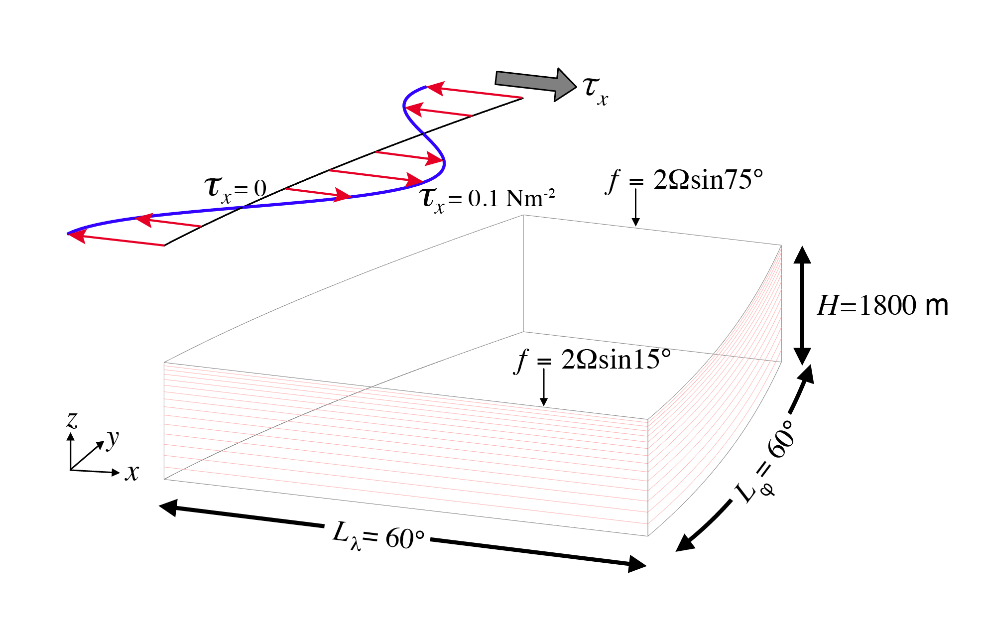
Schematic of simulation domain and wind-stress forcing function for baroclinic gyre numerical experiment. The domain is enclosed by solid walls. From MITgcm test case.

Forcing

The Coriolis parameter, $f$, is defined according to latitude $\phi$

$$f(\phi )=2\mathrm{\Omega }\sin (\phi )$$

with the rotation rate, $\mathrm{\Omega }$ set to $\frac{2\pi }{86164}{\text{s}}^{-1}$ (i.e., corresponding to the standard Earth rotation rate, using the CIME constant to ensure consistency). The sinusoidal wind-stress variations are defined according to

$${\tau }_{\lambda }(\phi )=-{\tau }_0\cos \left(2\pi \frac{\phi -{\phi }_o}{L_{\phi }}\right)$$

where $L_{\phi }$ is the lateral domain extent (${60}^{\circ }$), ${\phi }_o$ is set to ${15}^{\circ }\text{N}$ and ${\tau }_0$ is $0.1{\text{ N m}}^{-2}$. config options summarizes the configuration options used in this simulation.

Temperature is restored in the surface layer to a linear profile:

(1)$${\mathcal{F}}_{\theta }=-U_{piston}(\theta -{\theta }^{\ast }),\phantom{WWW}{\theta }^{\ast }=\frac{{\theta }_{\mathrm{m}\mathrm{a}\mathrm{x}}-{\theta }_{\mathrm{m}\mathrm{i}\mathrm{n}}}{L_{\phi }}({\phi }_{\mathrm{m}\mathrm{a}\mathrm{x}}-\phi )+{\theta }_{\mathrm{m}\mathrm{i}\mathrm{n}}$$

where the piston velocity $U_{piston}$ (in m.s^{-1}) is calculated by applying a relaxation timescale of 30 days (set in config file) over the thickness of the top layer (50 m by default) and ${\theta }_{\mathrm{m}\mathrm{a}\mathrm{x}}={30}^{\circ }$ C, ${\theta }_{\mathrm{m}\mathrm{i}\mathrm{n}}=0^{\circ }$ C.

Initial state

Initially the fluid is stratified with a reference potential temperature profile that varies from (approximately) $\theta =30.6{}^{\circ }$C in the surface layer to $\theta =1.56{}^{\circ }$C in the bottom layer. To ensure that the profile is independent of the vertical discretization, the profile is now set by a surface value (at the top interface) and a bottom value (at the bottom interface), set in the .cfg file. The default values have been chosen for the layer values (calculated with zMid) to approximate the discrete values presented in the MITgcm test case. The temperature functional form (and inner parameter cc was determined by fitting an analytical function to the MITgcm discrete layer values (originally ranging from 2 to $30{}^{\circ }$C. If the bottom_depth is different from the default 1800m value, the temperature profile is stretched in the vertical to fit the surface and bottom temperature constraints, but the thermocline depth and the discrete layer values will move away from the MITgcm test case. The equation of state used in this experiment is linear:

(2)$$\rho ={\rho }_0(1-{\alpha }_{\theta }{\theta }^{\prime })$$

with ${\rho }_0=999.8{\mathrm{k}\mathrm{g}\mathrm{m}}^{-3}$ and ${\alpha }_{\theta }=2\times {10}^{-4}{\mathrm{K}}^{-1}$. The salinity is set to a uniform value of $S=34$psu (set in the .cfg file) Given the linear equation of state, in this configuration the model state variable for temperature is equivalent to either in-situ temperature, $T$, or potential temperature, $\theta$. For simplicity, here we use the variable $\theta$ to represent temperature.

Analysis

For scientific validation, this test case is meant to be run to quasi-steady state and its mean state compared to the MITgcm test case and / or theoretical scaling. This is done through an analysis step in the 3_year_test case. Note that 3 years are likely insufficient to bring the test case to full equilibrium. Examples of qualitative plots include: i) equilibrated SSH contours on top of surface heat fluxes, ii) barotropic streamfunction (compared to MITgcm or a barotropic gyre test case).

Examples of checks against theory include: iii) max of simulated barotropic streamfunction ~ Sverdrup transport, iv) simulated thermocline depth ~ scaling argument for penetration depth (Vallis (2017) or Cushman-Roisin and Beckers (2011)).

Consider the Sverdrup transport:

$$\rho v_{\mathrm{b}\mathrm{t}}=\hat{\mathit{k}}\cdot \frac{\mathrm{\nabla }\times \overrightarrow{\mathit{\tau }}}{\beta }$$

If we plug in a typical mid-latitude value for $\beta$ ($2\times {10}^{-11}$ m^-1 s^-1) and note that $\tau$ varies by $0.1$ Nm² over ${15}^{\circ }$ latitude, and multiply by the width of our ocean sector, we obtain an estimate of approximately 20 Sv.

This scaling is obtained via thermal wind and the linearized barotropic vorticity equation), the depth of the thermocline $h$ should scale as:

$$h={\left(\frac{w_{\mathrm{E}\mathrm{k}}{f}^2{L}_x}{\beta \mathrm{\Delta }b}\right)}^2={\left(\frac{(\tau /L_y)f{L}_x}{\beta {\rho }^{\prime }}\right)}^2$$

where $w_{\mathrm{E}\mathrm{k}}$ is a representive value for Ekman pumping, $\mathrm{\Delta }b=g{\rho }^{\prime }/{\rho }_0$ is the variation in buoyancy across the gyre, and $L_x$ and $L_y$ are length scales in the $x$ and $y$ directions, respectively. Plugging in applicable values at ${30}^{\circ }$N, we obtain an estimate for $h$ of 200 m.

config options

All 2 test cases share the same set of config options:

# Options related to the vertical grid
[vertical_grid]

# the type of vertical grid
grid_type = linear_dz

# the linear rate of thickness (m) increase for linear_dz
linear_dz_rate = 10.

# Number of vertical levels
vert_levels = 15

# Total water column depth in m
bottom_depth = 1800.

# The type of vertical coordinate (e.g. z-level, z-star)
coord_type = z-star

# Whether to use "partial" or "full", or "None" to not alter the topography
partial_cell_type = None

# The minimum fraction of a layer for partial cells
min_pc_fraction = 0.1


# config options for the baroclinic gyre
[baroclinic_gyre]
# Basin dimensions
lat_min = 15
lat_max = 75
lon_min = 0
lon_max = 60

# Initial vertical temperature profile (C)
initial_temp_top = 33.
initial_temp_bot = 1.

# Constant salinity value (also used in restoring)
initial_salinity = 34.

# Maximum zonal wind stress value (N m-2)
wind_stress_max = 0.1

# Surface temperature restoring profile
restoring_temp_min = 0.
restoring_temp_max = 30.

# Restoring timescale for surface temperature (in days)
restoring_temp_timescale = 30.


# config options for the post processing (moc and viz)
[baroclinic_gyre_post]
# latitude bin increment for the moc calculation
dlat = 0.25
# number of years to average over for the mean state plots
time_averaging_length = 1

performance_test

ocean/baroclinic_gyre/performance_test is the default version of the baroclinic_gyre test case for a short (3 time steps) test run and validation of prognostic variables for regression testing.

3_year_test

ocean/baroclinic_gyre/3_year_test is an additional version of the baroclinic_gyre test case with a longer (3-year) spin-up. By default, it includes monthly mean output, and plots the mean state of the simulation for the last 1 year (option in the config file). Note that for the 80km configuration, the estimated time to equilibration is roughly 50 years (approx 3 hours of compute time on default layout). This can be done by running the forward step several times (adding 3 years each time), or by editing the forward/namelist.ocean file to set the config_run_duration to the desired simulation duration. For a detailed comparison of the mean state against theory and results from other models, the mean state at 100 years may be most appropriate to be aligned with the MITgcm results.