global_ocean¶

The ocean/global_ocean test group defines meshes, initial conditions, testing, and spin-up for global, realistic ocean domains. Currently, two mesh resolutions—QU240 and Icos240 and EC30to60, along with their variants with Ice-shelf cavities—have been ported from COMPASS legacy, with many more to follow in the coming months.

compass will be the tool used to create ocean meshes and initial conditions for future versions of E3SM.

The global_ocean test group a test case for creating each mesh, test cases for creating each of the 4 supported initial-conditions variants using that mesh, a number of test cases aimed at regression testing, and a spin-up test case for each mesh that produces an initial condition appropriate for incorporation into E3SM. (compass does not provide the tools for creating many of the files needed for full E3SM coupling, a process that requires expert help from the E3SM development team.)

Shared config options¶

All global_ocean test cases start the following shared config options. Note that meshes and test cases may modify these options, as noted below.

# options for spherical meshes
[spherical_mesh]

## config options related to the step for culling land from the mesh
# number of cores to use
cull_mesh_cpus_per_task = 128
# minimum of cores, below which the step fails
cull_mesh_min_cpus_per_task = 1
# maximum memory usage allowed (in MB)
cull_mesh_max_memory = 1000
# Whether to convert the culled mesh file to CDF5 format
convert_culled_mesh_to_cdf5 = False
# Minimum latitude, in degrees, for masking land-locked cells
latitude_threshold = 43.0
# Maximum number of sweeps to search for land-locked cells
sweep_count = 20


# Options relate to adjusting the sea-surface height or land-ice pressure
# below ice shelves to they are dynamically consistent with one another
[ssh_adjustment]

# the number of iterations of ssh adjustment to perform
iterations = 10

# Whether to convert adjusted initial condition files to CDF5 format during
# ssh adjustment under ice shelves
convert_to_cdf5 = False


# options for global ocean testcases
[global_ocean]

## each mesh should replace these with appropriate values in its config file

# the number of cells per core to aim for
goal_cells_per_core = 200
# the approximate maximum number of cells per core (the test will fail if too
# few cores are available)
max_cells_per_core = 2000

# the approximate number of cells in the mesh, to be estimated for each mesh
approx_cell_count = <<<Missing>>>

# time step per resolution (s/km), since dt is proportional to resolution
dt_per_km = 30
# barotropic time step per resolution (s/km)
btr_dt_per_km = 1.5

## config options related to the initial_state step

# minimum number of vertical levels, both in the open ocean and in ice-shelf
# cavities
min_levels = 3
cavity_min_levels = ${min_levels}

# minimum thickness of layers in ice-shelf cavities
cavity_min_layer_thickness = 1.0

# Maximum allowed Haney number for configurations with ice-shelf cavities
rx1_max = 20.0

# the number of iterations of topography smoothing (0 means no smoothing)
topo_smooth_num_passes = 0
# The distance in km over which the Gaussian filter is applied
topo_smooth_distance_limit = 200.0
# The standard deviation in km of the Gaussian filter
topo_smooth_std_deviation = 100.0

# number of cores to use
init_ntasks = 36
# minimum of cores, below which the step fails
init_min_tasks = 8
# number of threads
init_threads = 1
# The number of cores per task in init mode -- used to avoid running out of
# memory where needed
init_cpus_per_task = 1
# whether to update PIO tasks and stride
init_update_pio = True

## config options related to the forward steps
# number of threads
forward_threads = 1
# whether to update PIO tasks and stride
forward_update_pio = True

## metadata related to the mesh
# whether to add metadata to output files
add_metadata = True
# the prefix (e.g. QU, EC, WC, SO)
prefix = PREFIX
# a description of the mesh
mesh_description = <<<Missing>>>
# a description of the bathymetry
bathy_description = <<<Missing>>>
# a description of the mesh with ice-shelf cavities
init_description = <<<Missing>>>
# E3SM version that the mesh is intended for
e3sm_version = 3
# The revision number of the mesh, which should be incremented each time the
# mesh is revised
mesh_revision = <<Missing>>
# the minimum (finest) resolution in the mesh
min_res = <<<Missing>>>
# the maximum (coarsest) resolution in the mesh, can be the same as min_res
max_res = <<<Missing>>>
# the maximum depth of the ocean, always detected automatically
max_depth = autodetect
# the number of vertical levels, always detected automatically
levels = autodetect

# the date the mesh was created as YYYYMMDD, typically detected automatically
creation_date = autodetect
# The following options are detected from .gitconfig if not explicitly entered
author = autodetect
email = autodetect
# The URL of the pull request documenting the creation of the mesh
pull_request = <<<Missing>>>

# Elevation threshold for including land cells
floodplain_elevation = 10.0


# config options related to dynamic adjustment
[dynamic_adjustment]

# the maximum allowed value of temperatureMax in global statistics
temperature_max = 33.0


# config options related to initial condition and diagnostics support files
# for E3SM
[files_for_e3sm]

# The minimum and maximum cells per core for creating graph partitions
max_cells_per_core = 30000
min_cells_per_core = 2

## the following relate to the comparison grids in MPAS-Analysis to generate
## mapping files for.  The default values are also the defaults in
## MPAS-Analysis.  Coarser or finer resolution may be desirable for some MPAS
## meshes.

# The comparison lat/lon grid resolution in degrees
comparisonLatResolution = 0.5
comparisonLonResolution = 0.5

# The comparison Antarctic polar stereographic grid size and resolution in km
comparisonAntarcticStereoWidth = 6000.
comparisonAntarcticStereoResolution = 10.

# The comparison Arctic polar stereographic grid size and resolution in km
comparisonArcticStereoWidth = 6000.
comparisonArcticStereoResolution = 10.

# The extended Antarctic polar stereographic comparison grid size and
# resolution in km
comparisonAntarcticExtendedWidth = 9000.
comparisonAntarcticExtendedResolution = 15.

# The extended Arctic polar stereographic comparison grid size and
# resolution in km
comparisonArcticExtendedWidth = 9000.
comparisonArcticExtendedResolution = 15.

# The comparison North Atlantic grid size and resolution in km
comparisonNorthAtlanticWidth = 8500.
comparisonNorthAtlanticHeight = 5500.
comparisonNorthAtlanticResolution = 20.

# The comparison North Pacific c grid size and resolution in km
comparisonNorthPacificWidth = 15000.
comparisonNorthPacificHeight = 5000.
comparisonNorthPacificResolution = 20.

# The comparison North Atlantic grid size and resolution in km
comparisonSubpolarNorthAtlanticWidth = 7000.
comparisonSubpolarNorthAtlanticHeight = 4000.
comparisonSubpolarNorthAtlanticResolution = 20.

# CMIP6 grid resolution
cmip6_grid_res = 180x360

# the E3SM short name of the mesh or "autodetect" to use the
# MPAS_Mesh_Short_Name attribute of the mesh file
mesh_short_name = autodetect

# the absolute path or relative path with respect to the test case's work
# directory of an ocean restart file on the given mesh
ocean_restart_filename = autodetect

# the base mesh before culling for remapping and rerouting data ice-shelf melt
# fluxes
ocean_base_mesh_filename = autodetect

# the initial state used to extract the ocean and sea-ice meshes
ocean_initial_state_filename = ${ocean_restart_filename}

# the absolute path or relative path with respect to the test case's work
# directory of a graph file that corresponds to the mesh
graph_filename = autodetect

# whether the mesh has ice-shelf cavities
with_ice_shelf_cavities = autodetect

# whether to write out sea-ice partition info for plotting in paraview
plot_seaice_partitions = False

The cull_mesh_*, init_* and forward:* config options are used to specify the resources used in in the mesh step of the mesh test case, the initial_state step of the init test case and the Forward step, respectively. These values will differ between test cases and meshes.

The next group of config options (add_metadata to pull_request) specify metadata related to the mesh and initial condition. These will be filled in based on the mesh and initial condition of the particular test case.

The final group are used in the files_for_e3sm test case.

Metadata¶

Most global_ocean test cases produce output files in NetCDF format. The MPAS development team decided in April 2020 to add a standardized set of metadata to these files to document the mesh and initial condition, and to provide provenance describing the environment used to create the mesh.

compass adds the following fields to most NetCDF files (those related to the initial condition are not added to mesh files, because the initial condition is not yet known at the time of mesh creation):

:MPAS_Mesh_Short_Name = "QU240E2r1" ;
:MPAS_Mesh_Long_Name = "QU240kmL16E3SMv2r1" ;
:MPAS_Mesh_Prefix = "QU" ;
:MPAS_Mesh_E3SM_Version = "2" ;
:MPAS_Mesh_Pull_Request = "https://github.com/MPAS-Dev/compass/pull/28" ;
:MPAS_Mesh_QU_Revision = "1" ;
:MPAS_Mesh_QU_Version_Author = "Xylar Asay-Davis" ;
:MPAS_Mesh_QU_Version_Author_E-mail = "xylar@lanl.gov" ;
:MPAS_Mesh_QU_Version_Creation_Date = "210116" ;
:MPAS_Mesh_QU_Minimum_Resolution_km = "240" ;
:MPAS_Mesh_QU_Maximum_Resolution_km = "240" ;
:MPAS_Mesh_QU_Maximum_Depth_m = "3000.0" ;
:MPAS_Mesh_QU_Number_of_Levels = "16" ;
:MPAS_Mesh_Description = "MPAS quasi-uniform mesh for E3SM version 2 at 240-km global resolution with 16 vertical level" ;
:MPAS_Mesh_Bathymetry = "Bathymetry is from GEBCO 2022, combined with BedMachine Antarctica v2 around Antarctica." ;
:MPAS_Initial_Condition = "Polar science center Hydrographic Climatology (PHC)" ;
:MPAS_Mesh_COMPASS_Version = "1.0.0" ;
:MPAS_Mesh_JIGSAW_Version = "0.9.12" ;
:MPAS_Mesh_JIGSAW-Python_Version = "0.2.1" ;
:MPAS_Mesh_MPAS-Tools_Version = "0.2.0" ;
:MPAS_Mesh_NCO_Version = "4.9.7" ;
:MPAS_Mesh_ESMF_Version = "8.0.1" ;
:MPAS_Mesh_geometric_features_Version = "0.1.13" ;
:MPAS_Mesh_Metis_Version = "5.1.0" ;
:MPAS_Mesh_pyremap_Version = "0.0.8" ;

Most of these options can be modified by the user by editing config options. The most convenient way to do this is to add them to the user config file when you are Setting up test cases or Test Suites. In particular, you may wish to set:

# options for global ocean testcases
[global_ocean]

## metadata related to the mesh
# whether to add metadata to output files
add_metadata = True
# the date the mesh was created as YYMMDD, typically detected automatically
creation_date = autodetect
# The following options are detected from .gitconfig if not explicitly entered
author = autodetect
email = autodetect
# The URL of the pull request documenting the creation of the mesh
pull_request = <<<Missing>>>

Meshes¶

The process for creating global ocean meshes is described below in the mesh test case. compass currently supports 5 meshes. Two are at such coarse horizontal resolution (240 km) that they are mostly useful for testing purposes, not scientific simulations. Two more meshes, which vary in resolution between 30 and 60 km, are used as the lowest resolution meshes in E3SM’s science campaigns. The final mesh has resolution focused in the Southern Ocean around Antarctica.

QU240 and Icos240¶

The quasi-uniform 240-km (QU240) mesh, is a global mesh with approximately 240-km horizontal resolution everywhere (as the name implies). The Icos240 mesh is similar but based on a subdivided icosahedron, and thus has grid cells that are more regular in size and shape. Ice-shelf cavities around Antarctica are excluded from the mesh. This mesh is used as part of the nightly test suite to perform regression and performance testing in a coarse but realistic model configuration. This mesh is also being used in studies of climate reproducibility.

QUwISC240 and IcoswISC240¶

The quasi-uniform 240-km mesh with ice-shelf cavities (QUwISC240) and the corresponding icosahedral mesh (IcoswISC240) are nearly identical to the QU240 and Icos240 meshes except that they include the Ice-shelf cavities around Antarctica in the ocean domain.

MPAS-Ocean’s treatment of ice-shelf cavities requires and iterative adjustment step to make the landIcePressure compatible with the ssh (see Sea surface height adjustment). This process is relatively time consuming, requiring a short forward run for each iteration, meaning that QUwISC240 is less efficient for regression and performance testing than QU240. However, it is useful for low-resolution testing that exercises compass and MPAS-Ocean functionality related to ice-shelf cavities and sub-ice-shelf freshwater fluxes.

QU, Icos, QUwISC and IcoswISC¶

The quasi-uniform (QU) and icosahedral (Icos) general meshes are global meshes with approximately constant horizontal resolution everywhere. As with all global ocean meshes, if wISC is in the mesh name, Ice-shelf cavities around Antarctica are included, otherwise they are excluded. The resolution of the mesh is determined by a user config file, with a default of 120 km (very low resolution). In addition to config options related to the vertical grid and metadata, the only important config option for these meshes is:

# options for global ocean testcases
[global_ocean]

# the resolution of the QU or Icos mesh in km
qu_resolution = 120

You can specify qu_resolution by placing it in a user config file and modify it before setting up test cases with the QU mesh. You could also modify the config option in each test case after setting them up but this is typically too tedious to be practical.

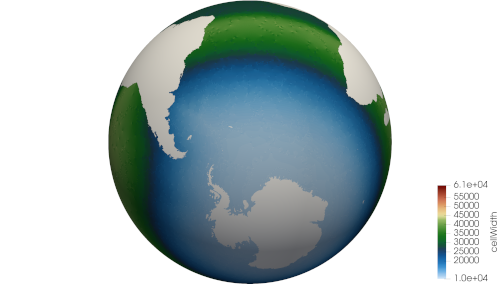
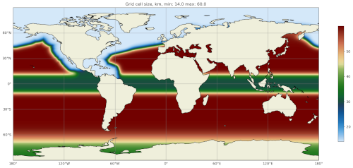
EC30to60¶

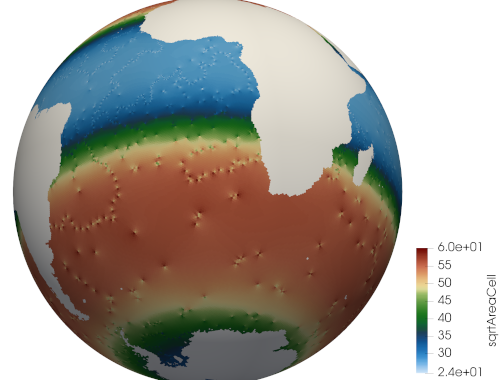
The eddy-closure 30- to 60-km (EC30to60) mesh is the coarsest MPAS-Ocean mesh used for scientific simulations. It is coarse enough that it requires the Gent-McWilliams eddy closure <https://doi.org/10.1175/1520-0485(1990)020<0150:IMIOCM>2.0.CO;2> as a parameterization of mixing from mesoscale ocean eddies.

The image above shows the resolution (as measured by \(\sqrt{A_c}\), where \(A_c\) is the area of a cell in the mesh). The resolution is approximately zonally invariant and transitions smoothly between three target resolutions as a function of latitude: ~30 km at around the equator, ~60 km at mid-latitudes and ~35 km near the the poles.

ECwISC30to60¶

The eddy-closure 30- to 60-km mesh with ice-shelf cavities (ECwISC30to60) is nearly identical to the EC30to60 except that it includes the Ice-shelf cavities around Antarctica in the ocean domain.

A variant of this mesh has been used for low resolution simulations as part of the E3SM v1 Cryosphere Campaign.

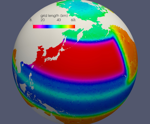
Kuroshio8to60 and Kuroshio12to60¶

The Kuroshio 8- and 12- to 60-km meshes (Kuroshio8to60 and Kuroshio12to60) are designed to explore dynamics of the Kuroshio Current.

The meshes have 8 and 12 km resolution, respectively, in the western North Pacific, tapering to 60 km at mid latitudes, 30 km at the equator, and 35 km in polar regions (the same as the EC30to60).

RRS6to18 and RRSwISC6to18¶

The E3SM v3 high resolution meshes are the Rossby-radius-scaling (RRS) 6- to 18-km meshes. They have resolution that scales as a function of latitude approximately with the Rossby radius of deformation from 6 km at the poles to 18 km at the equator. The RRSwISC6to18 mesh has ice-shelf cavities around Antarctica, whereas the RRS6to18 mesh does not.

SO12to60 and SOwISC12to60¶

The Southern Ocean 12- to 60-km mesh with ice-shelf cavities (SOwISC12to60), sometimes called the Southern Ocean regionally refined mesh (SORRM), is the main simulation mesh for the E3SM v2 Cryosphere Science Campaign and E3SM v3 Polar Processes, Sea-Level Rise, and Coastal Impacts Campaign.

The SO12to60 is the same mesh but without ice-shelf cavities. The mesh has 12 km resolution around Antarctica, tapering to 45 km in mid Southern latitudes, 30 km at the equator and in the North Atlantic, 60 km in the North Pacific, and 35 km in the Arctic. The mesh includes the Ice-shelf cavities around Antarctica in the ocean domain.

WC14 and WCwISC14¶

The Water Cycle 14- to 60-km mesh (WC14) is intended to be the main regionally refined simulation mesh for the E3SM v2 Water Cycle Science Campaign. The E3SM v3 Water Cycle Changes and Impacts Campaign is expected to use the same mesh but including ice-shelf cavities (WCwISC14).

The mesh has 14 km resolution around the continental US, Arctic Ocean and parts of the North Atlantic, tapering to 60 km in mid latitudes, 30 km at the equator, and 35 km around Antarctica.

Ice-shelf cavities¶

As discussed in Ice shelf-cavities, the inclusion of ice-shelf cavities and melt rates below ice shelves around Antarctica is a major objective of the E3SM Cryosphere Campaign.

Each of the global_ocean Meshes can support a variant with ice-shelf cavities along with one without. Meshes with cavities include the wISC suffix for “with ice-shelf cavities” attached to the mesh prefix (e.g. QU or EC). Currently all meshes include both variants but we anticipate that future meshes may include only the variant with or without cavities.

Around Antarctica, the topographic data currently used to construct initial conditions in compass comes from BedMachineAntarctica. Because this data set provides the ice draft, rather than the weight of the overlying ice shelf, we use the method for Sea surface height adjustment to update the pressure from the ice shelf to be in dynamic balance with the ice draft.

Forward step¶

The only step shared across many global_ocean test cases is forward (though I doesn’t always go by that name), which integrates the MPAS-Ocean model in time in “forward” mode.

As a user, your main way of altering forward runs is by changing namelist options directly in namelist.ocean or modifying streams in streams.ocean. However, there are a few parameters related to forward runs you can change in the config file for a test case. Since some test cases like restart_test test case and :ref`global_ocean_dynamic_adjustment` have more than one forward run, it is convenient to change options like forward_ntasks once in the config file, knowing that this will change the target number of cores of all forward model runs in the test case. The same applies to the other forward_* config options that change the minimum cores allowed, the number of threads, and (in the future) the maximum memory and disk usage.

Test cases¶

global_ocean includes 9 types of test cases (each with different versions for different meshes, initial conditions, time integrators, etc.).

mesh test case¶

The ocean/global_ocean/<mesh>/mesh test case (where <mesh> is the name of a mesh, e.g. QU240 and Icos240) creates a “base” horizontal mesh covering the globe with a distribution of resolution according to the specifications of the mesh. The base mesh is created using the JIGSAW and JIGSAW-Python tools. Then, a mask for “land” (i.e. non-ocean) cells is created and the mesh is culled so that only ocean cells are retained. The data set determining which cells are land vs. ocean depends on whether ice-shelf cavities are included in the mesh or not (see Ice-shelf cavities). A coastline from Natural Earth is combined with either the edge of Antarctic Ice Sheet (AIS) or the edge of the grounded portion of the AIS from BedMachineAntarctica. These coastlines come from the geometric_features package.

For most meshes, tools and data sets from the geometric_features and from the mpas_tools package are used to ensure that some transects such the thin opening at Gibraltar connecting the Mediterranean Sea to the Atlantic Ocean (so-called “critical passages”) are represented by contiguous ocean cells while others such as the Antarctic Peninsula (so-called “critical land blockages”) are blocked by land with no ocean connectivity.

As part of culling the mesh, adding critical passages, and removing critical land blockages, there is also a step in which a “flood fill” is performed to ensure that all parts of the global ocean are connected to one another by at least one neighboring cell.

init test case¶

Once the horizontal mesh has been created, the next step is to create a vertical mesh and and initial condition.

The default vertical coordinate depends on the mesh being used, as described in Meshes. Possible grid types are described in Vertical coordinate and include uniform, tanh_dz, index_tanh_dz, 60layerPHC, 80layerE3SMv1, and 100layerE3SMv1.

compass supports 3 different types of initial conditions. One is the World Ocean Atlas 2023 (WOA23) climatology from 1991-2020. The second is derived from the Polar science center Hydrographic Climatology (PHC). The last is the UK MetOffice’s EN4 estimated climatology for the year 1900 (EN4_1900).

All subsequent tests (performance_test test case, restart_test test case, etc.) could potentially start from any of these initial conditions, meaning that a performance test starting from WOA23 should be thought of as a different test from one starting from PHC. Therefore, it is convenient to house the init test case and all subsequent test cases that depend on it within a subdirectory with the name of the initial condition. The relative paths associate with each initial condition for a given <mesh> are:

ocean/global_ocean/<mesh>/WOA23/init
ocean/global_ocean/<mesh>/PHC/init
ocean/global_ocean/<mesh>/EN4_1900/init

For meshes with ice-shelf cavities, init also interpolates the Paolo et al. (2023) annual mean Antarctic melt rates to the MPAS mesh for use in subsequent test cases and possible incorporation as a forcing dataset in E3SM. The init test case also performs an ssh_adjustment step as described in Sea surface height adjustment.

performance_test test case¶

The performance_test test case runs 1 or 2 short forward integration, then performs validation of prognostic variables (layer thickness, velocity, temperature and salinity) and, if applicable, variables related to fluxes below ice shelves. The duration of the forward run depends on the mesh and the time integrator.

Depending on the mesh, versions of the test may exist with both or either of the split-explict (base on Higdon 2005) or the 4th-order Runge-Kutta (RK4) time integrator. Each of these possible variants is given its own subdirectory. Thus, for a given mesh <mesh> and initial condition <ic>, one or more of these versions of the performance_test will be available:

ocean/global_ocean/<mesh>/<ic>/performance_test/split_explicit
ocean/global_ocean/<mesh>/<ic>/performance_test/RK4

Versions of this test cases is currently available for all meshes, but not necessarily for all combinations of initial conditions and time integrators.

If ice-shelf cavities are not present, the test case includes 1 forward step.

In configurations with ice-shelf cavities, the test performs 2 short forward runs, one with prognostic ice-shelf melt fluxes and one with “data” ice shelf melt fluxes derived from satellite observations.

restart_test test case¶

The restart_test test case runs a short forward integration, saving an intermediate restart file. Then, in a second forward step, the test continues the run from the restart file. Output from the two steps (full_run and restart_run) are compared to make sure prognostic variables (layer thickness, velocity, temperature and salinity) are unchanged.

As with the performance_test test case, restart_test can be run with either or both of the split-explicit or RK4 time integrator. Thus, for a the QU240 and Icos240 or QUwISC240 and IcoswISC240 mesh (currently the only supported meshes) and initial condition <ic>, one or more of these versions of the restart_test will be available:

ocean/global_ocean/QU240/<ic>/restart_test/split_explicit
ocean/global_ocean/QU240/<ic>/restart_test/RK4
ocean/global_ocean/QUwISC240/<ic>/restart_test/split_explicit
ocean/global_ocean/QUwISC240/<ic>/restart_test/RK4

decomp_test test case¶

The decomp_test test case runs a short forward integration with 4 cores (4proc) and then performs the same run again in another step with 8 cores (8proc). Prognostic variables (layer thickness, velocity, temperature and salinity) are compared to make sure they are unchanged.

As with the performance_test test case, decomp_test can be run with either or both of the split-explicit or RK4 time integrator. Thus, for a the QU240 and Icos240 or QUwISC240 and IcoswISC240 mesh (currently the only supported meshes) and initial condition <ic>, one or more of these versions of the decomp_test will be available:

ocean/global_ocean/QU240/<ic>/decomp_test/split_explicit
ocean/global_ocean/QU240/<ic>/decomp_test/RK4
ocean/global_ocean/QUwISC240/<ic>/decomp_test/split_explicit
ocean/global_ocean/QUwISC240/<ic>/decomp_test/RK4

threads_test test case¶

The threads_test test case runs a short forward integration with 1 thread and 4 cores (1thread) and then performs the same run again in another step with 2 threads and 4 cores (2thread). Prognostic variables (layer thickness, velocity, temperature and salinity) are compared to make sure they are unchanged.

As with the performance_test test case, threads_test can be run with either or both of the split-explicit or RK4 time integrator. Thus, for a the QU240 and Icos240 or QUwISC240 and IcoswISC240 mesh (currently the only supported meshes) and initial condition <ic>, one or more of these versions of the threads_test will be available:

ocean/global_ocean/QU240/<ic>/threads_test/split_explicit
ocean/global_ocean/QU240/<ic>/threads_test/RK4
ocean/global_ocean/QUwISC240/<ic>/threads_test/split_explicit
ocean/global_ocean/QUwISC240/<ic>/threads_test/RK4

analysis_test test case¶

The analysis_test is used to test the proper function and validate the output from a large number of MPAS-Ocean’s “analysis members”. Analysis members allow MPAS-Ocean to compute analysis during the model run, meaning much of the same infrastructure and functionality used in the forward model can also be used for analysis. Analysis members are also useful for analysis that is too large or time consuming to perform after the simulation has completed, or where storing the required data to disk would be infeasible.

The analysis members tested in this test case are:

globalStats
surfaceAreaWeightedAverages
waterMassCensus
layerVolumeWeightedAverage
zonalMean
okuboWeiss
meridionalHeatTransport
highFrequencyOutput
eliassenPalm
mixedLayerDepths
debugDiagnostics
eddyProductVariables
oceanHeatContent
mixedLayerHeatBudget

For more information on these analysis members, see the MPAS-Ocean user’s guide.

As with the performance_test test case, analysis_test can be run with either or both of the split-explicit or RK4 time integrator. Thus, for a the QU240 and Icos240 or QUwISC240 and IcoswISC240 mesh (currently the only supported meshes) and initial condition <ic>, one or more of these versions of the analysis_test will be available:

ocean/global_ocean/QU240/<ic>/analysis_test/split_explicit
ocean/global_ocean/QU240/<ic>/analysis_test/RK4
ocean/global_ocean/QUwISC240/<ic>/analysis_test/split_explicit
ocean/global_ocean/QUwISC240/<ic>/analysis_test/RK4

daily_output_test test case¶

The daily_output_test is similar to the analysis_test test case: it is used to run and validate the timeSeriesStatsDaily analysis member. The reason for a separate test is that the daily_output_test must run for a full day to produce useful output, significantly longer than the analysis_test test case.

The timeSeriesStatsDaily performs daily averages of a large number of model variables. The variables in this test are kept in sync with the default output of the timeSeriesStatsMonthly analysis member used in E3SM. This test is used to gain confidence that E3SM output from MPAS-Ocean will have the expected variables and formatting. For example, the test is currently being used in an effort to improve compliance to the CF Conventions <https://cfconventions.org/> in the output metadata.

As with the performance_test test case, daily_output_test can be run with either or both of the split-explicit or RK4 time integrator. Thus, for a the QU240 and Icos240 or QUwISC240 and IcoswISC240 mesh (currently the only supported meshes) and initial condition <ic>, one or more of these versions of the daily_output_test will be available:

ocean/global_ocean/QU240/<ic>/daily_output_test/split_explicit
ocean/global_ocean/QU240/<ic>/daily_output_test/RK4
ocean/global_ocean/QUwISC240/<ic>/daily_output_test/split_explicit
ocean/global_ocean/QUwISC240/<ic>/daily_output_test/RK4

dynamic_adjustment test case¶

One of the main purposes of compass is to provide a way of spinning up MPAS-Ocean initial conditions to dissipate transients that result from starting the simulation from rest. Particularly for high resolution meshes, surface waves with fast time scales and large amplitude must be damped (by applying Rayleigh friction), first aggressively, then more gently, before damping is disabled.

The dynamic_adjustment test case is implemented differently for each of the Meshes. For example, for the QU240 and Icos240 and ref:global_ocean_mesh_quwisc240 meshes, we perform only 1 day of damping (and even this is likely unnecessary), followed by a 1-day simulation without damping. In contrast, for the EC30to60 and ref:global_ocean_mesh_ecwisc30to60 meshes, we perform a 10-day spin-up with aggressive damping, followed by 10 more days without damping. Higher resolution meshes in Legacy COMPASS require several stages of damping, each over several days before damping can be removed.

Currently dynamic_adjustment is only available for the split-explicit (not the RK4) time integrator. Thus, for a given mesh <mesh> and initial condition <ic>, the dynamic_adjustment will be available at:

ocean/global_ocean/<mesh>/<ic>/dynamic_adjustment

Versions of this test cases is currently available for all meshes, but not necessarily for all combinations of initial conditions and time integrators.

The qu240_for_e3sm test suite, quwisc240_for_e3sm test suite, ec30to60 test suite and ecwisc30to60 test suite are Test suites designed to make it easier to run the standard dynamic-adjustment test cases for each mesh along with the related mesh test case, init test case, and files_for_e3sm test case.

files_for_e3sm test case¶

After running the dynamic_adjustment test case, users may be interested in preparing a number of files needed for including a new mesh in E3SM. These files include: MPAS-Ocean and MPAS-Seaice initial conditions (including Metadata); SCRIP files; partition files, created with gpmetis, for splitting the mesh across a number of possible core counts; a mask file for MPAS-Ocean’s mocStreamfunction analysis member; mask and mapping files for MPAS-Analysis; and a file containing data ice-shelf melt rates for running DISMF (data ice-shelf melt flux) compsets in E3SM.

The resulting files are symlinked in a subdirectory of the test case called assembled_files. This directory contains subdirectories with the same structure as the E3SM data server. For new meshes, these files can be uploaded by an expert from the E3SM team along with additional files required for full E3SM integration. Currently, there is not a way to use new meshes in E3SM without help from an expert from the E3SM team.

files_for_e3sm for an existing mesh¶

Sometimes, we already have an E3SM initial condition but some of the support files, such as the diagnostics files for MPAS-Analysis or the graph partition files for MPAS-Seaice, either weren’t created with the initial condition or they are out of date. The ocean/global_ocean/files_for_e3sm test case is useful for creating these files.

The user should create local symlinks to an E3SM initial condition, a graph file, and a base-mesh file for MPAS-Ocean for the desired mesh. Then, the config options in files_for_e3sm.cfg should be edited. In this example, we have created a local link to the mpaso.IcoswISC30E3r5.20231120.nc initial condition and the mpas-o.graph.info.20231120 graph file in the test case directory. We also created a symlink to the base mesh (found in the share/meshes/mpas/ocean subdirectory within the inputdata diretory on a given E3SM supported machine). The mesh name has also been set to the E3SM short name for this mesh IcoswISC30E3r5. We indicate that the mesh includes ice-shelf cavities, which means we include processing related to ice-shelf melt rates.

We also need to provide several options in the [global_ocean] section of the config file so the metadata added to the initial conditions will be correct.

 [global_ocean]

 prefix = Icos

mesh_description = MPAS subdivided icosahedral mesh for E3SM version
                  ${e3sm_version} at ${min_res}-km global resolution with
                  <<<levels>>> vertical level

 bathy_description = Bathymetry is from GEBCO 2023, combined with
                     BedMachine Antarctica v3 around Antarctica.

 init_description = World Ocean Atlas 2023 climatology 1991-2020

 e3sm_version = 3
 mesh_revision = 5
 min_res = 30
 max_res = 30
 pull_request = https://github.com/MPAS-Dev/compass/pull/735
 creation_date = 20240219
 author = Xylar Asay-Davis
 email = xylar@lanl.gov

 [files_for_e3sm]

 mesh_short_name = IcoswISC30E3r5
 ocean_restart_filename = mpaso.IcoswISC30E3r5.20231120.nc
 ocean_base_mesh_filename = IcoswISC30E3r5_base.20240219.nc
 graph_filename = mpas-o.graph.info.20231120
 with_ice_shelf_cavities = True

The resulting files are symlinked in a subdirectory of the test case called assembled_files. This directory contains subdirectories with the same structure as the E3SM data server. These files can be uploaded by an expert from the E3SM team. We ask that users not try to upload the files themselves without consulting an expert from the team.