buttermilk_bay¶

The buttermilk_bay test group implements a realistic regional simulation of tidally forced circulation in a multi-bay system connected by narrow channels. The computational domain is Buttermilk Bay, Massachusetts.

default¶

The default test case implements the Buttermilk Bay test case found in Kennedy et al. (2019). The tidal forcing is applied to a portion of the bottom boundary with an amplitude of 2 m and a period of 0.5 days.

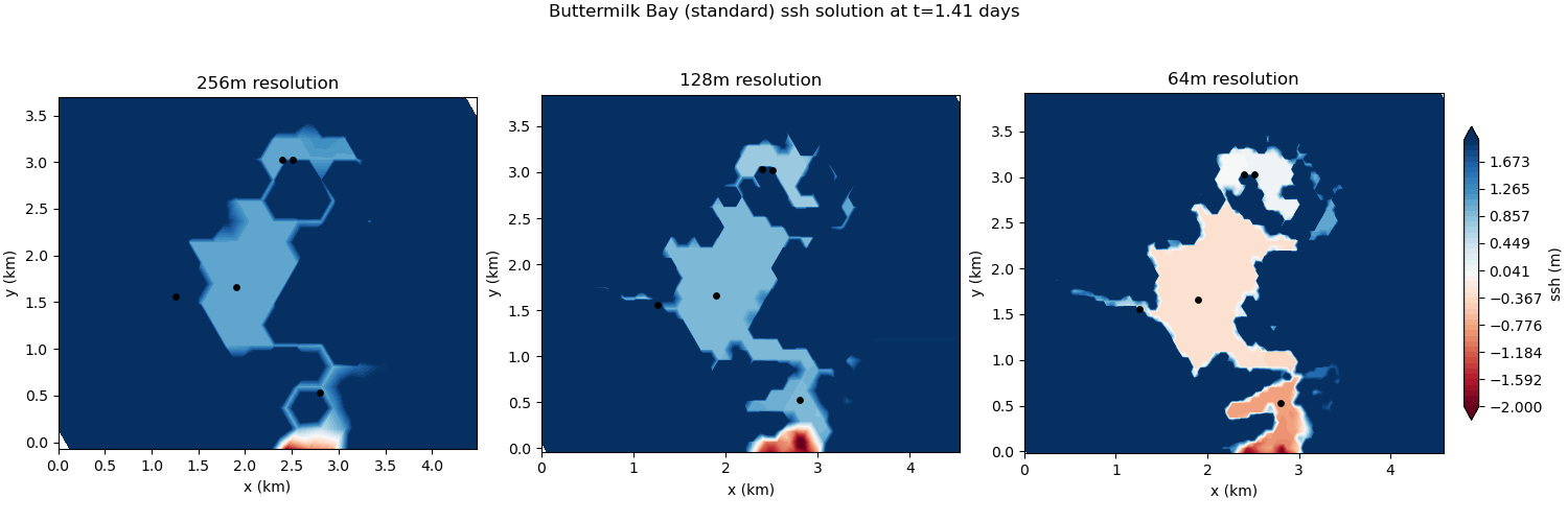
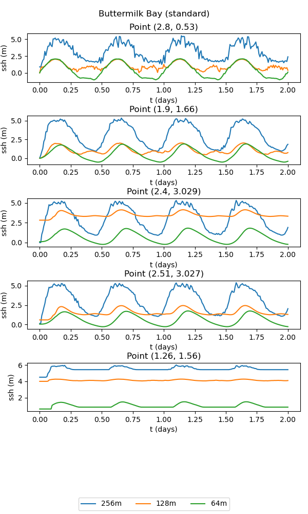
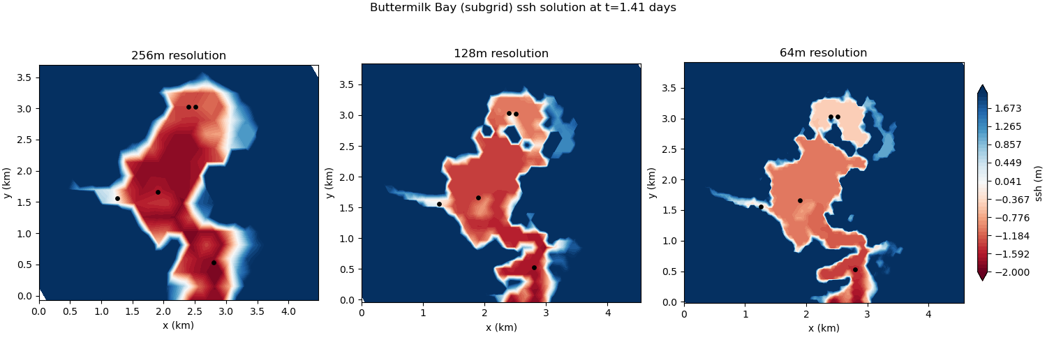
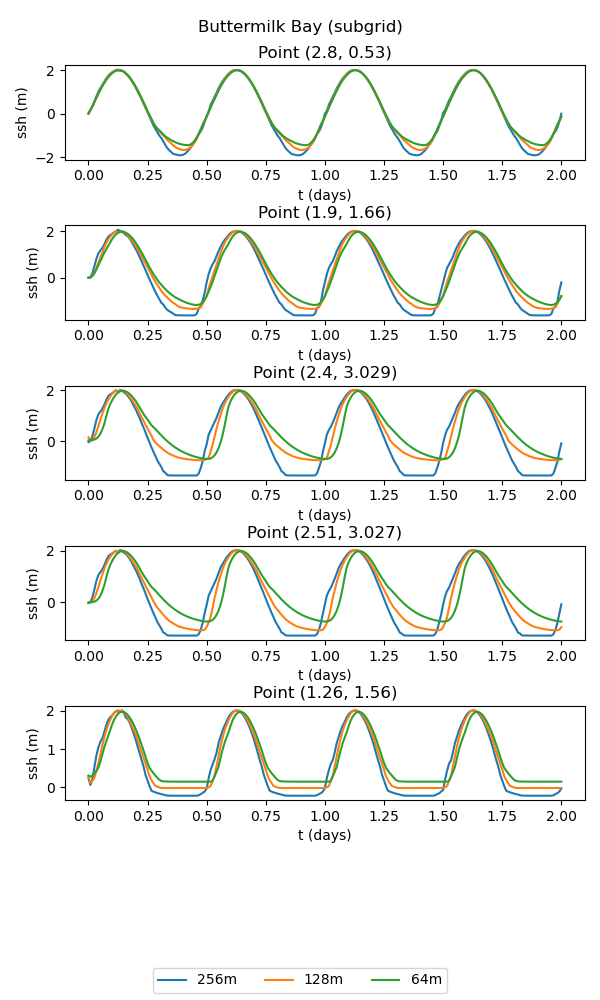
By default, the resolution is varied from 256 m to 64 m by doubling the resolution, with the time step proportional to resolution. The wetting/drying ramp feature (config_zero_drying_velocity_ramp = .true.) is used by default for both the standard and subgrid versions of this test case. The result of the viz step of the test case is plots of the solution at different times, a time series at various points, and a convergence plot.

standard¶

The standard version of the test case uses the standard wetting and drying approach. At coarser resolutions, the bathymetric representation lacks sufficient detail to resolve the connectivity between the upper and lower bays. As a consequence, the results of the simulation are quite poor:

../../../_images/buttermilk_bay_standard_points.png

subgrid¶

The subgrid version of the test case includes a subgrid correction scheme to incorporate the effects of subgrid scale bathymetric variations on the flow. This allows the small-scale connectivity between bays to be represented, leading to significant improvements over the standard wetting and drying approach:

../../../_images/buttermilk_bay_subgrid_points.png

config options¶

The buttermilk_bay config options include:

# config options for buttermilk bay
[buttermilk_bay]

# dimensions of domain in x and y directions (m)
Lx = 4608
Ly = 4608

# a list of resolutions (m) to test
resolutions = 256, 128, 64

# time step per resolution (s/m), since dt is proportional to resolution
dt_per_m = 0.02

# the number of cells per core to aim for
goal_cells_per_core = 300

# the approximate maximum number of cells per core (the test will fail if too
# few cores are available)
max_cells_per_core = 3000

# config options for visualizing drying slope ouptut
[buttermilk_bay_viz]

# coordinates (in km) for timeseries plot
points = [2.8, 0.53], [1.9, 1.66], [2.4, 3.029], [2.51, 3.027], [1.26, 1.56]

# generate contour plots at a specified interval between output timesnaps
plot_interval = 1

resolutions¶

The default resolutions (in m) used in the test case are:

resolutions = 256, 128, 64

To alter the resolutions used in this test, you will need to create your own config file (or add a buttermilk_bay section to a config file if you’re already using one). The resolutions are a comma-separated list of the resolution of the mesh in meters. If you specify a different list before setting up buttermilk_bay, steps will be generated with the requested resolutions. (If you alter resolutions in the test case’s config file in the work directory, nothing will happen.) The resolution value along the values of Lx and Ly are used to determine the number of cells in the x and y directions used to generate the mesh.

time step¶

The time step for forward integration is determined by multiplying the resolution by dt_per_m, so that coarser meshes have longer time steps. You can alter this before setup (in a user config file) or before running the test case (in the config file in the work directory).

cores¶

The number of cores (and the minimum) is proportional to the number of cells, so that the number of cells per core is roughly constant. You can alter how many cells are allocated to each core with goal_cells_per_core. You can control the maximum number of cells that are allowed to be placed on a single core (before the test case will fail) with max_cells_per_core. If there aren’t enough processors to handle the finest resolution, you will see that the step (and therefore the test case) has failed.

viz¶

The visualization step can be configured to plot the timeseries for an arbitrary set of coordinates by setting points. By default, these are set to the locations used in Kennedy et al. 2019. Also, the interval between contour plot time snaps can be controlled with plot_interval.