parabolic_bowl

The parabolic_bowl test group implements convergence study for wetting and drying. Currently, the only test case is the default case

default

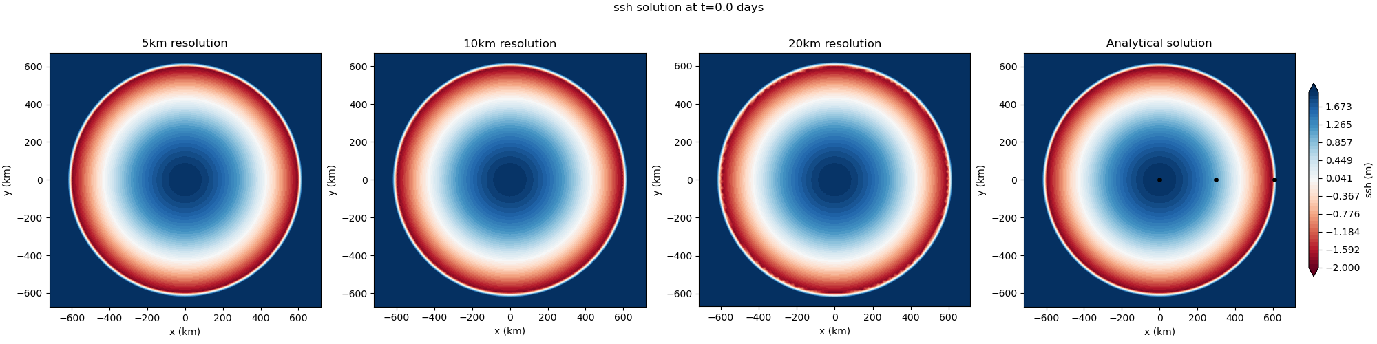
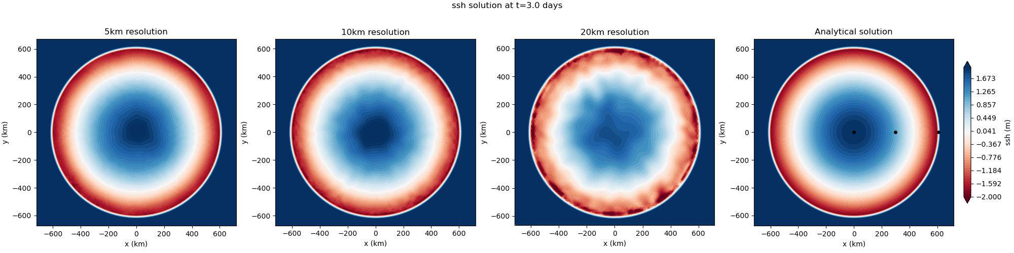
The default test case implements the parabolic bowl test case found in Thacker 1981. The problem consists an initial mound of water which propagates outward and reflects off a wet/dry boundary in a parabolic-shaped basin. The presence of a Coriolis factor causes the wave to rotate around the bowl as it oscillates. The bathymetry is given as:

\[b(x,y) = b_0\left(1 - \frac{R^2}{L^2}\right),\]

with

\[\begin{split}R &= \sqrt{x^2 + y^2}, \\ L &= \sqrt{\frac{8gb_0}{\omega^2 - f^2}}.\end{split}\]

An exact solution for this problem exists for the frictionless, nonlinear shallow water equations:

\[\begin{split}\eta(x,y,t) &= b_0\left[ \frac{\sqrt{1-C^2}}{1-C\cos(\omega t)} -1 - \left( \frac{R^2}{L^2} \right)\left( \frac{1-C^2}{(1-C\cos(\omega t))^2}-1\right)\right], \\ u(x,y,t) &= \frac{1}{1-C\cos(\omega t)}\left( \frac{1}{2}\omega x C \sin(\omega t) - \frac{1}{2}fy\left( \sqrt{1-C^2} + C\cos(\omega t) - 1\right)\right), \\ v(x,y,t) &= \frac{1}{1-C\cos(\omega t)}\left(\frac{1}{2}fx\left(\sqrt{1-C^2} + A\cos(\omega t) -1 \right) + \frac{1}{2}\omega y C \sin(\omega t)\right),\end{split}\]

where, \(C\) is defined as:

\[C = \frac{(b_0+\eta_0)^2 - b_0^2}{(b_0+\eta_0)^2 + b_0^2}.\]

Since this is a single layer case, the solution for the total depth, \(h = \eta + b\), is

\[h(x,y,t) = b_0\left[ \frac{\sqrt{1-C^2}}{1-C\cos(\omega t)} - \left( \frac{R^2}{L^2} \right)\left( \frac{1-C^2}{(1-C\cos(\omega t))^2}\right)\right].\]

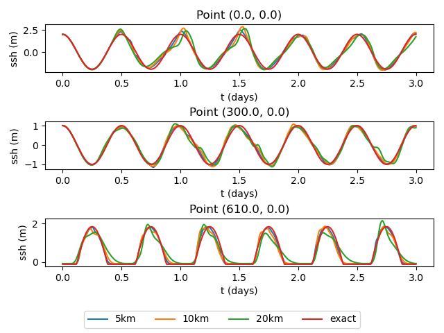
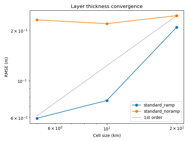
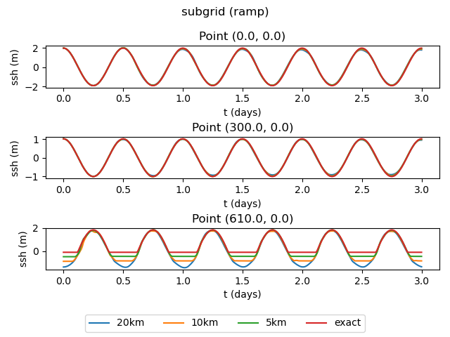
By default, the resolution is varied from 20 km to 5 km by doubling the resolution, with the time step proportional to resolution. The result of the viz step of the test case is are plots of the solution at different times, a time series at various points, and a convergence plot.

lts

Both the ramp and noramp test cases can be run with the lts variant which uses local time-stepping (LTS) as time integrator. Note that the tests verify the ability of the LTS scheme to run correctly with wetting and drying and are not designed to leverage the LTS capability of producing faster runs.

subgrid

Both the ramp and noramp test cases can be run with a subgrid scale correction scheme that accounts for the effects of subgrid scale flow in partially wet cells due to fine-scale bathymetric variation. This approach is useful becuase it allows connectivity due to unresolved features to be represented. In many coastal applications, this scheme can enable coarse resolution models to capture flooding with accuracy comprable to what higher-resolution simulations achieve without the subgrid corrections. 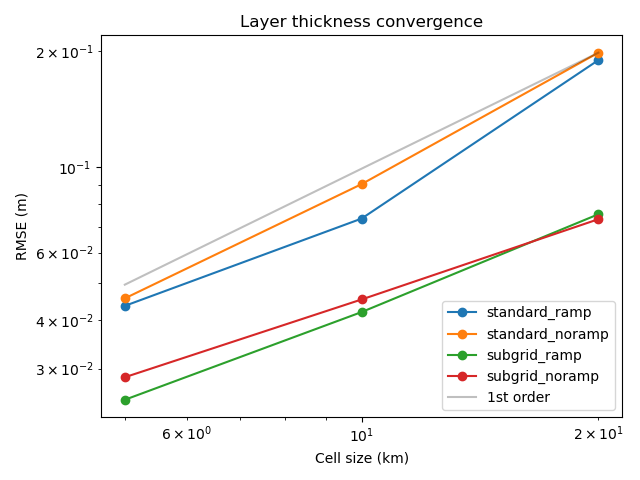Using the subgrid corrections for the parabolic bowl should result in reduced errors vs. using only the standard wetting and drying. For more details on the subgrid scale correction scheme see: Kennedy et al. (2019). Results for the subgrid test cases are shown below:

config options

The parabolic_bowl config options include:

# config options for drying slope test cases
[parabolic_bowl]

# dimensions of domain in x and y directions (km)
Lx = 1440
Ly = 1560

# Coriolis parameter
coriolis_parameter = 1.031e-4

# Maximum initial ssh magnitude
eta_max = 2.0

# Maximum water depth
depth_max = 50.0

# Angular fequency of oscillation
omega = 1.4544e-4

# Gravitational acceleration
gravity = 9.81

# a list of resolutions (km) to test
resolutions = 20, 10, 5

# time step per resolution (s/km), since dt is proportional to resolution
dt_per_km = 0.5

# the number of cells per core to aim for
goal_cells_per_core = 300

# the approximate maximum number of cells per core (the test will fail if too
# few cores are available)
max_cells_per_core = 3000

# config options for visualizing drying slope ouptut
[parabolic_bowl_viz]

# coordinates (in km) for timeseries plot
points = [0,0], [300,0], [610,0]

# generate contour plots at a specified interval between output timesnaps
plot_interval = 10

The first 6 options are used to control properties of the initial/analytical solution. The remaining options are discussed below.

resolutions

The default resolutions (in km) used in the test case are:

resolutions = 20, 10, 5

To alter the resolutions used in this test, you will need to create your own config file (or add a parabolic_bowl section to a config file if you’re already using one). The resolutions are a comma-separated list of the resolution of the mesh in km. If you specify a different list before setting up parabolic_bowl, steps will be generated with the requested resolutions. (If you alter resolutions in the test case’s config file in the work directory, nothing will happen.)

time step

The time step for forward integration is determined by multiplying the resolution by dt_per_km, so that coarser meshes have longer time steps. You can alter this before setup (in a user config file) or before running the test case (in the config file in the work directory).

cores

The number of cores (and the minimum) is proportional to the number of cells, so that the number of cells per core is roughly constant. You can alter how many cells are allocated to each core with goal_cells_per_core. You can control the maximum number of cells that are allowed to be placed on a single core (before the test case will fail) with max_cells_per_core. If there aren’t enough processors to handle the finest resolution, you will see that the step (and therefore the test case) has failed.

viz

The visualization step can be configured to plot the timeseries for an arbitrary set of coordinates by setting points. Also, the interval between contour plot time snaps can be controlled with plot_interval. An error convergence plot is also generated. Errors for the ramp and noramp cases for both the standard and subgrid cases, if the output exists at the time it is run.