climatologyMapCustom

An analysis task for plotting custom climatologies at various depths. This task can plot both 2D and 3D variables on cells, the latter with both nVertlevels – layer centers – or nVertLevelsP1 – layer interfaces – as the vertical dimension. The task is designed to be highly coustomizable via config sections and options, as described below.

Component and Tags:

component: ocean
tags: climatology, horizontalMap

Configuration Options

The following configuration options are available for this task:

[climatologyMapCustom]
## options related to plotting climatology maps of any field at various depths
## (if they include a depth dimension) without observatons for comparison

# comparison grid(s)
comparisonGrids = ['latlon']

# Months or seasons to plot (Jan, Feb, Mar, Apr, May, Jun, Jul, Aug, Sep, Oct,
# Nov, Dec, JFM, AMJ, JAS, OND, ANN)
seasons =  ['ANN']

# list of depths in meters (positive up) at which to analyze, 'top' for the
# sea surface, 'bot' for the sea floor
depths = ['top', -200, -400, -600, -800, -1000, -1500, -2000, 'bot']

# a list of variables available to plot. New variables can be added as long
# as they correspond to a single field already found in MPAS-Ocean's
# timeSeriesStatsMonthly output. Add the 'name', 'title', 'units' (with $$
# instead a single dollar sign for the config parser), and 'mpas'(the
# timeSeriesStatsMonthly variable name as a single-item list) entries for each
# variable. Then, add a section below climatologyMapCustom<VariableName> with
# the colormap settings for that variable.
availableVariables = {
    'temperature':
        {'title': 'Potential Temperature',
        'units': r'$$^\circ$$C',
        'mpas': ['timeMonthly_avg_activeTracers_temperature']},
    'salinity':
        {'title': 'Salinity',
        'units': 'PSU',
        'mpas': ['timeMonthly_avg_activeTracers_salinity']},
    'potentialDensity':
        {'title': 'Potential Density',
        'units': 'kg m$$^{-3}$$',
        'mpas': ['timeMonthly_avg_potentialDensity']},
    'thermalForcing':
        {'title': 'Thermal Forcing',
        'units': r'$$^\circ$$C',
        'mpas': ['timeMonthly_avg_activeTracers_temperature',
                'timeMonthly_avg_activeTracers_salinity',
                'timeMonthly_avg_density',
                'timeMonthly_avg_activeTracers_layerThickness']},
    'zonalVelocity':
        {'title': 'Zonal Velocity',
        'units': r'm s$$^{-1}$$',
        'mpas': ['timeMonthly_avg_velocityZonal']},
    'meridionalVelocity':
        {'title': 'Meridional Velocity',
        'units': r'm s$$^{-1}$$',
        'mpas': ['timeMonthly_avg_velocityMeridional']},
    'velocityMagnitude':
        {'title': 'Zonal Velocity',
        'units': r'm s$$^{-1}$$',
        'mpas': ['timeMonthly_avg_velocityZonal',
                'timeMonthly_avg_velocityMeridional']},
    'vertVelocity':
        {'title': 'Vertical Velocity',
        'units': r'm s$$^{-1}$$',
        'mpas': ['timeMonthly_avg_vertVelocityTop']},
    'vertDiff':
        {'title': 'Vertical Diffusivity',
        'units': r'm s$$^{-1}$$',
        'mpas': ['timeMonthly_avg_vertDiffTopOfCell']},
    'vertVisc':
        {'title': 'Vertical Viscosity',
        'units': r'm s$$^{-1}$$',
        'mpas': ['timeMonthly_avg_vertViscTopOfCell']},
    'mixedLayerDepth':
        {'title': 'Mixed Layer Depth',
        'units': 'm',
        'mpas': ['timeMonthly_avg_dThreshMLD']},
    }

# a list of fields top plot for each transect.  All supported fields are listed
# below
variables = []


[climatologyMapCustomTemperature]
## options related to plotting climatology maps of potential temperature at
## various levels, including the sea surface and sea floor, possibly against
### control model results

# colormap for model/observations
colormapNameResult = RdYlBu_r
# whether the colormap is indexed or continuous
colormapTypeResult = continuous
# the type of norm used in the colormap
normTypeResult = linear
# A dictionary with keywords for the norm
normArgsResult = {'vmin': -2., 'vmax': 10.}
# place the ticks automatically by default
# colorbarTicksResult = numpy.linspace(-2., 10., 9)

# colormap for differences
colormapNameDifference = balance
# whether the colormap is indexed or continuous
colormapTypeDifference = continuous
# the type of norm used in the colormap
normTypeDifference = linear
# A dictionary with keywords for the norm
normArgsDifference = {'vmin': -5., 'vmax': 5.}
# place the ticks automatically by default
# colorbarTicksDifference = numpy.linspace(-5., 5., 9)

[climatologyMapCustomSalinity]
colormapNameResult = haline
colormapTypeResult = continuous
normTypeResult = linear
normArgsResult = {'vmin': 32.2, 'vmax': 35.5}
colormapNameDifference = balance
colormapTypeDifference = continuous
normTypeDifference = linear
normArgsDifference = {'vmin': -1.5, 'vmax': 1.5}

[climatologyMapCustomPotentialDensity]
colormapNameResult = Spectral_r
colormapTypeResult = continuous
normTypeResult = linear
normArgsResult = {'vmin': 1026.5, 'vmax': 1028.}
colormapNameDifference = balance
colormapTypeDifference = continuous
normTypeDifference = linear
normArgsDifference = {'vmin': -0.3, 'vmax': 0.3}

[climatologyMapCustomThermalForcing]
colormapNameResult = thermal
colormapTypeResult = continuous
normTypeResult = linear
normArgsResult = {'vmin': -1., 'vmax': 5.}
colormapNameDifference = balance
colormapTypeDifference = continuous
normTypeDifference = linear
normArgsDifference = {'vmin': -3., 'vmax': 3.}

[climatologyMapCustomZonalVelocity]
colormapNameResult = delta
colormapTypeResult = continuous
normTypeResult = linear
normArgsResult = {'vmin': -0.2, 'vmax': 0.2}
colormapNameDifference = balance
colormapTypeDifference = continuous
normTypeDifference = linear
normArgsDifference = {'vmin': -0.2, 'vmax': 0.2}

[climatologyMapCustomMeridionalVelocity]
colormapNameResult = delta
colormapTypeResult = continuous
normTypeResult = linear
normArgsResult = {'vmin': -0.2, 'vmax': 0.2}
colormapNameDifference = balance
colormapTypeDifference = continuous
normTypeDifference = linear
normArgsDifference = {'vmin': -0.2, 'vmax': 0.2}

[climatologyMapCustomVelocityMagnitude]
colormapNameResult = ice
colormapTypeResult = continuous
normTypeResult = log
normArgsResult = {'vmin': 1.e-3, 'vmax': 1.}
colormapNameDifference = balance
colormapTypeDifference = continuous
normTypeDifference = linear
normArgsDifference = {'vmin': -0.2, 'vmax': 0.2}

[climatologyMapCustomVertVelocity]
colormapNameResult = delta
colormapTypeResult = continuous
normTypeResult = linear
normArgsResult = {'vmin': -1e-5, 'vmax': 1e-5}
colormapNameDifference = balance
colormapTypeDifference = continuous
normTypeDifference = linear
normArgsDifference = {'vmin': -1e-5, 'vmax': 1e-5}

[climatologyMapCustomVertDiff]
colormapNameResult = rain
colormapTypeResult = continuous
normTypeResult = log
normArgsResult = {'vmin': 1e-6, 'vmax': 1.}
colormapNameDifference = balance
colormapTypeDifference = continuous
normTypeDifference = linear
normArgsDifference = {'vmin': -0.5, 'vmax': 0.5}

[climatologyMapCustomVertVisc]
colormapNameResult = rain
colormapTypeResult = continuous
normTypeResult = log
normArgsResult = {'vmin': 1e-6, 'vmax': 1.}
colormapNameDifference = balance
colormapTypeDifference = continuous
normTypeDifference = linear
normArgsDifference = {'vmin': -0.5, 'vmax': 0.5}

[climatologyMapCustomMixedLayerDepth]
colormapNameResult = viridis
colormapTypeResult = continuous
normTypeResult = log
normArgsResult = {'vmin': 10., 'vmax': 300.}
colorbarTicksResult = [10, 20, 40, 60, 80, 100, 200, 300]
colormapNameDifference = balance
colormapTypeDifference = continuous
normTypeDifference = symLog
normArgsDifference = {'linthresh': 10., 'linscale': 0.5, 'vmin': -200.,
                    'vmax': 200.}
colorbarTicksDifference = [-200., -100., -50., -20., -10., 0., 10., 20., 50., 100., 200.]

There is a section for options that apply to all custom climatology maps and one each for any available variables to plot.

The option availableVariables is a dictionary with the names of the variables available to plot as keys and dictionaries with the title, units, and MPAS variable name(s) as values. New entries can be added as long as they correspond to a single field already found in MPAS-Ocean’s timeSeriesStatsMonthly output. For each variable, a section with the name climatologyMapCustom<VariableName> should be added with the colormap settings for that variable, see Colormaps for details.

The option depths is a list of (approximate) depths at which to sample the potential temperature field. A value of 'top' indicates the sea surface (or the ice-ocean interface under ice shelves) while a value of 'bot' indicates the seafloor.

By default, no fields are plotted. A user can select which fields to plot by adding the desired field names to the variables list.

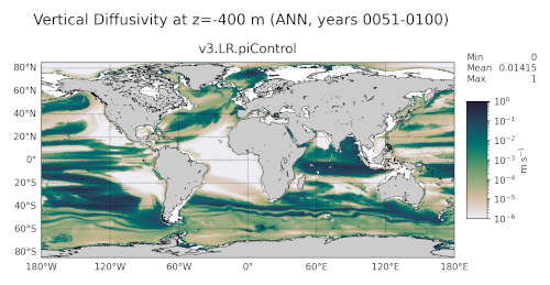
For more details, see:

• Colormaps

• Seasons

• Comparison Grids

Example Result