conservation
An analysis task for plotting histograms of 2-d variables of climatologies in ocean regions.
Component and Tags:
component: ocean
tags: timeseries, conservation
Configuration Options
The following configuration options are available for this task:
[conservation]
## options related to producing time series plots, often to compare against
## observations and previous runs
# the year from which to compute anomalies if not the start year of the
# simulation. This might be useful if a long spin-up cycle is performed and
# only the anomaly over a later span of years is of interest.
# anomalyRefYear = 249
# start and end years for timeseries analysis. Use endYear = end to indicate
# that the full range of the data should be used. If errorOnMissing = False,
# the start and end year will be clipped to the valid range. Otherwise, out
# of bounds values will lead to an error. In a "control" config file used in
# a "main vs. control" analysis run, the range of years must be valid and
# cannot include "end" because the original data may not be available.
startYear = 1
endYear = end
# Plot types to generate. The following plotTypes are supported:
# total_energy_flux : Total energy flux
# absolute_energy_error : Energy error
# ice_salt_flux : Salt flux related to land ice and sea ice
# absolute_salt_error : Salt conservation error
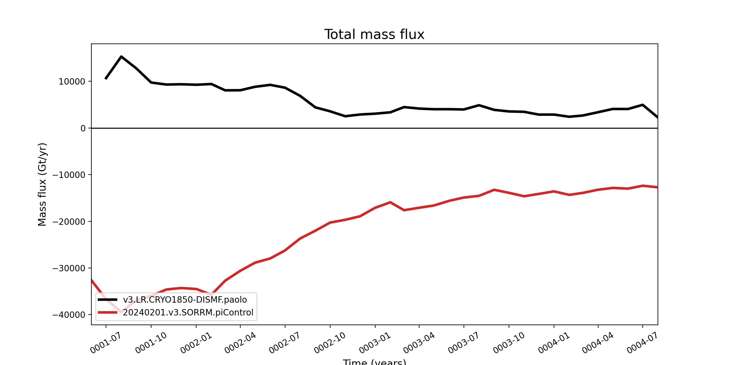
# total_mass_flux : Total mass flux
# total_mass_change : Total mass anomaly
# land_ice_mass_change : Mass anomaly due to land ice fluxes
# land_ice_ssh_change : SSH anomaly due to land ice fluxes
# land_ice_mass_flux_components : Mass fluxes from land ice
plotTypes = 'land_ice_mass_flux_components'
# line colors for the main, control and obs curves
# see https://matplotlib.org/stable/gallery/color/named_colors.html
# and https://matplotlib.org/stable/tutorials/colors/colors.html
mainColor = black
controlColor = tab:red
Example Result