timeSeriesOHCAnomaly
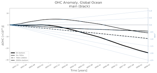
An analysis task for plotting a Hovmoller plot (time and depth axes) and depth-integrated time series of the anomaly in ocean heat content (OHC) from a reference year (usually the first year of the simulation).
Component and Tags:
component: ocean
tags: timeSeries, ohc, publicObs
Configuration Options
The following configuration options are available for this task:
[timeSeriesOHCAnomaly]
## options related to plotting time series of ocean heat content (OHC)
## anomalies from year 1

# list of regions to plot from the region list in [regions] below
regions = ['global']

# approximate depths (m) separating plots of the upper, middle and lower ocean
depths = [700, 2000]

# preprocessed file prefix, with format OHC.<preprocessedRunName>.year*.nc
preprocessedFilePrefix = OHC

# prefix on preprocessed field name, with format ohc_<suffix> for suffixes
# 'tot', '700m', '2000m', 'btm'
preprocessedFieldPrefix = ohc

# Number of points over which to compute moving average(e.g., for monthly
# output, movingAveragePoints=12 corresponds to a 12-month moving average
# window)
movingAveragePoints = 12

# An optional first year for the tick marks on the x axis. Leave commented out
# to start at the beginning of the time series.
# firstYearXTicks = 1

# An optional number of years between tick marks on the x axis.  Leave
# commented out to determine the distance between ticks automatically.
# yearStrideXTicks = 1

[hovmollerOHCAnomaly]
## options related to time vs. depth Hovmoller plots of ocean heat content
## (OHC) anomalies from year 1

# Note: regions and moving average points are the same as for the time series
# plot

# colormap
colormapName = balance
# colormap indices for contour color
colormapIndices = [0, 28, 57, 85, 113, 142, 170, 198, 227, 255]
# colorbar levels/values for contour boundaries
colorbarLevels = [-2.4, -0.8, -0.4, -0.2, 0, 0.2, 0.4, 0.8, 2.4]
# contour line levels
contourLevels = np.arange(-2.5, 2.6, 0.5)

# An optional first year for the tick marks on the x axis. Leave commented out
# to start at the beginning of the time series.

# firstYearXTicks = 1

# An optional number of years between tick marks on the x axis.  Leave
# commented out to determine the distance between ticks automatically.
# yearStrideXTicks = 1
For the depth-integrated time-series plot, the user may select the depths (in meters) that separate the upper, middle and lower regions of the ocean, e.g.:
depths = [700, 2000]
indicates that OHC will be integrated from 0 to 700 m, 700 to 2000 m, and 2000 m to the ocean floor (as well as from 0 to the ocean floor).
The OHC can be compared with results from a reference v0 simulation. If
preprocessedRunName in the [runs] section is not None, the
depth integrated time series will be read in with a file prefix given by
preprocessedFilePrefix and a field prefix given by
preprocessedFieldPrefix. Generally, these options should not be altered
except of debugging purposes.
Recently, a right-hand axis and an associated set of lines has been added to the OHC anomaly time series. This axis and these lines show the equivalent top-of-atmosphere energy flux (\(W/m^2\)) that the ocean heat anomaly would induce.
- For more details on other config options, see:
Example Result